Introduction

Training deep neural networks presents several challenges related to memory constraints, computational resources, and convergence issues. This document explores advanced techniques that address these challenges, including optimization algorithms like Stochastic Gradient Descent (SGD), SGD with Momentum, Adam, LARS, and LAMB, as well as methods such as gradient accumulation and activation checkpointing.

Optimizing the Loss Function in Machine Learning

Definition: Optimizing a loss function in machine learning involves finding the set of model parameters that minimizes the discrepancy between the model’s predicted outputs and the actual target values in the training data.

Purpose: The loss function provides a single scalar value that quantifies how well the model’s predictions align with the true values, guiding the optimization process.

Fundamental Concepts

Optimization in Machine Learning

General Form:

\[
w^* = \arg \min_{w} L(w) = \arg \min_{w} \frac{1}{N} \sum_{i=1}^N l(f(x_i; w_i), y_i)
\]

• \( f(x_i; w_i) \): Model’s prediction for input \( x_i \)
• \( y_i \): True label
• \( l(\cdot, \cdot) \): Loss function measuring the discrepancy between prediction and true label
• \( N \): Number of training examples

Types of Optimization Problems

1. Convex Optimization

• Characteristics:
  Global Minimum Guarantee: In convex optimization, the objective function is convex, ensuring any local minimum is also a global minimum. This makes algorithms like gradient descent reliable in finding the best solution.
• Convex Function:
  A function \( f(w) \) is convex if the line segment between any two points on the graph lies above the graph. Mathematically, \( f(w) \) is convex if for all \( w_1, w_2 \) and \( \lambda \) in the range [0, 1]:
  \[
  f(\lambda w_1 + (1 – \lambda) w_2) \leq \lambda f(w_1) + (1 – \lambda) f(w_2)
  \]
• Example:
  Linear Regression with Mean Squared Error (MSE) Loss: Linear regression minimizes the MSE between predicted and actual values, a convex function that ensures efficient convergence to the global minimum.

2. Non-Convex Optimization

• Characteristics:
  Multiple Local Minima: Non-convex optimization problems have objective functions with multiple local minima and maxima, making it challenging to find the global minimum as algorithms might get stuck in local minima.
• Non-Convex Function:
  A function \( f(w) \) is non-convex if it does not satisfy the convexity condition, leading to an optimization landscape with multiple valleys (local minima) and peaks (local maxima).
• Example:
  Neural Network Training: Optimizing the loss function in neural networks is a non-convex problem due to the complex loss surface, which includes many local minima and saddle points. This complexity arises from the nonlinear activation functions and the large number of parameters. Specialized algorithms and techniques like momentum and adaptive learning rates are often employed to navigate these challenges.

Challenges in Optimization

• Ill-conditioning: Occurs when the condition number of the Hessian of the loss function is large, leading to slow convergence.
• Saddle Points: Points where the gradient is zero but are neither a local minimum nor a maximum.
• Plateaus: Regions where the gradient is close to zero across a wide range of parameter values.
• Stochasticity: Noise in gradient estimates when using mini-batches.

Common Loss Functions

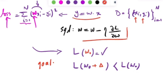
1. Mean Squared Error (MSE) for Regression

\[
\text{MSE} = \frac{1}{N} \sum_{i=1}^N (y_i – \hat{y}_i)^2
\]

• \( N \): Total number of data points.
• \( y_i \): Actual value for the \( i \)-th data point.
• \( \hat{y}_i \): Predicted value for the \( i \)-th data point.

2. Cross-Entropy Loss for Classification

• Binary Cross-Entropy Loss:

\[
\text{Loss} = -\frac{1}{N} \sum_{i=1}^N \left[ y_i \log(\hat{y}_i) + (1 – y_i) \log(1 – \hat{y}_i) \right]
\]

• \( N \): The total number of data points in the dataset.
• \( y_i \): The actual binary indicator (0 or 1) for the \( i \)-th data point.
• \( \hat{y}_i \): The predicted probability that the \( i \)-th data point  data point (ranging between 0 and 1).

• Multiclass Cross-Entropy Loss:

\[
\text{Loss} = -\frac{1}{N} \sum_{i=1}^N \sum_{c=1}^C y_{i,c} \log(\hat{y}_{i,c})
\]

• \( N \): The total number of data points in the dataset.
• \( C \): The total number of classes.
• \( y_{i,c} \): The actual binary indicator (0 or 1) if class label \( c \) is the correct classification for the \( i \)-th data point.
• \( \hat{y}_{i,c} \): The predicted probability that the \( i \)-th data point belongs to class \( c \).

Steps for Optimizing a Loss Function

1. Define the Loss Function: Choose an appropriate loss function for the task.
2. Initialize Model Parameters: Start with initial values for the model parameters, which could be set randomly or based on some heuristic.
3. Forward Pass: Use the current model parameters to make predictions on the training data.
4. Compute Loss: Calculate the loss using the loss function by comparing the model’s predictions to the actual target values.
5. Backward Pass: Compute the gradients of the loss with respect to the model parameters using techniques like backpropagation.
6. Update Parameters: Adjust the model parameters in the direction that reduces the loss using optimization algorithms.
7. Iterate: Repeat the forward pass, loss computation, backward pass, and parameter update steps for multiple iterations (epochs) until the loss converges to a minimum value or stops improving significantly.
8. Evaluate: Assess the optimized model on a separate validation or test dataset to ensure it generalizes well to unseen data.

Optimization Methods

First-Order Methods

First-order methods involve computing the gradient of the loss function with respect to the model parameters. The gradient indicates the direction of the steepest ascent. For minimization purposes, the parameters are adjusted in the opposite direction of the gradient.

• Key Component: Gradient of the loss function.
• Example: Gradient Descent.

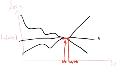
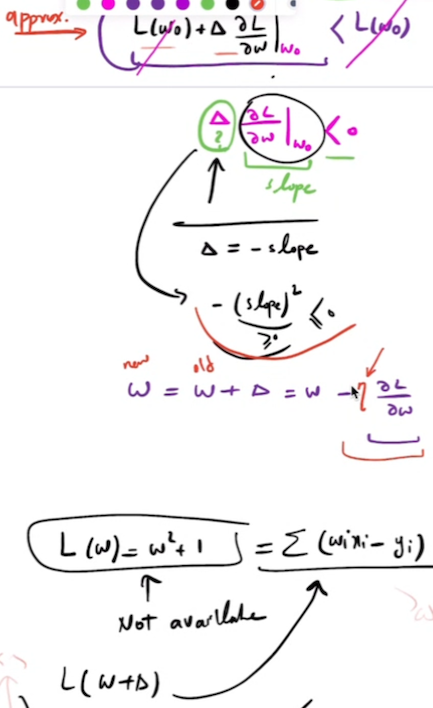
Stochastic Gradient Descent (SGD)

• SGD Update Rule: SGD updates the parameters w of a model to minimize a loss function L(w). The update rule for SGD is typically based on the gradient of the loss function:

\[
w_{t+1} = w_t – \eta \nabla L(w_t)
\]

where:

• \(w_{t+1} \) is the parameter vector at iteration \( t \),
• \(\eta \) is the learning rate,
• \(\nabla L(w_t) \) is the gradient of the loss function with respect to the parameters.

• Deriving the Gradient Using Central Difference Approximation: The Central Difference Approximation can be used to derive the Stochastic Gradient Descent (SGD) equation by approximating the gradient (derivative) of the loss function with respect to the parameters. Given a function \( f(x) \), the derivative \( f'(x) \) at a point \( x \) can be approximated using the Central Difference Approximation as:

\[
\frac{\partial L(w_t)}{\partial w_i} \approx \frac{L(w_t + h e_i) – L(w_t – h e_i)}{2h}
\]

where:

• \( e_i \) is a unit vector with 1 in the \( i \)-th position and 0 elsewhere,
•  \( h i\) s a small value.

• SGD with Central Difference Approximation: Substituting the central difference approximation into the SGD update rule gives

\[
w_{t+1} = w_t – \eta \frac{L(w_t + h e_i) – L(w_t – h e_i)}{2h}
\]

This equation shows how SGD can be performed using a numerical approximation of the gradient instead of calculating the exact analytical gradient. In practice, this approach is computationally more expensive than using the true gradient, so it is typically used only for checking or when the gradient is difficult to compute analytically.

Second-Order Methods

Second-order methods utilize the Hessian matrix (second derivative) to provide information about the curvature of the loss function.

Second-order methods utilize the second derivative, or Hessian matrix, to provide information about the curvature of the loss function. The nature of the Hessian at a critical point determines whether the point is a local minimum, local maximum, or a saddle point:

• If the Hessian is positive definite, the point is a local minimum.
• If the Hessian is negative definite, the point is a local maximum.
• If the Hessian has mixed signs, the point is a saddle point.
• Key Component: Second derivative (Hessian matrix)
• Advantage: Provides information about the curvature, determining whether a critical point is a local minimum, maximum, or saddle point.

Adaptive Learning Rates

Adaptive learning rates refer to a class of optimization algorithms that dynamically adjust the learning rate for each parameter during training. These algorithms leverage the statistical properties of the gradients, specifically the first and second moments, to adapt the learning rates, improving convergence and performance.

• Key Concept: Dynamic adjustment of learning rates.
• Example Algorithms: Adam, RMSprop.

Understanding First and Second Moments in Optimization Algorithms

In optimization, particularly for training neural networks, advanced algorithms leverage the concepts of moments to enhance the performance of gradient-based methods. These moments are used to stabilize and accelerate convergence by adjusting updates based on past gradients.

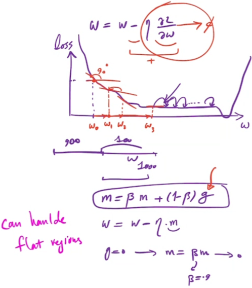
First Moment (Mean of the Gradients)

Concept Overview

• Gradient Descent Basics:
  Gradient descent updates model parameters in the direction opposite to the gradient of the loss function. While effective, this can lead to oscillations or slow convergence, especially in regions where gradients change direction frequently.
• Role of the First Moment:
  To address these issues, optimization algorithms use the first moment to smooth the gradient updates. The first moment is an exponentially weighted moving average of past gradients, which stabilizes the update direction.

Mathematical Representation

The first moment \( m_{t+1} \) at iteration \( t \) is updated using:

\[ m_{t+1} = \beta_1 m_t + (1 – \beta_1) \nabla L(w_t) \]

where:

• \( m_{t+1} \): Smoothed gradient estimate at time step \( t+1 \).
• \( \beta_1 \): Smoothing parameter, typically close to 1 (e.g., 0.9).
• \( m_t \): First moment estimate from the previous time step.
• \( \nabla L(w_t) \): Gradient of the loss function at time step \( t \).

Interpretation and Benefits

• Smoothing Gradient Estimates:
  The first moment provides a smoothed estimate of the gradient, reducing the effect of noisy or abrupt gradient changes. This results in more stable and consistent updates.
• Exponential Moving Average:
  By giving more weight to recent gradients, the first moment adjusts to recent changes while maintaining stability from past gradients.
• Practical Advantages:
  • Reduced Oscillations: The smoothed gradient reduces oscillations and provides a more consistent update direction.
  • Faster Convergence: Helps in accelerating convergence by smoothing out the gradient noise, making the optimization process more efficient.

Second Moment (Variance of the Gradients)

Concept Overview

• Variance of Gradients:
  The second moment refers to the uncentered variance or the average of the squared gradients. It provides insight into the magnitude of the gradients and is used to scale the learning rate.

Mathematical Representation

The second moment \( v_{t+1} \) at iteration \( t \) is updated as:

\[ v_{t+1} = \beta_2 v_t + (1 – \beta_2) (\nabla L(w_t))^2 \]

where:

• \( v_{t+1} \): Estimate of the variance of the gradients at time step \( t+1 \).
• \( \beta_2 \): Smoothing parameter for the second moment, usually close to 1 (e.g., 0.999).
• \( v_t \): Second moment estimate from the previous time step.
• \( (\nabla L(w_t))^2 \): Squared gradient of the loss function at time step \( t \).

Interpretation and Benefits

• Scaling Learning Rates:
  The second moment adjusts the learning rate based on the magnitude of the gradients. Large gradients result in a smaller learning rate to prevent overshooting, while small gradients result in a larger learning rate to speed up convergence.
• Stability and Adaptivity:
  By considering the variability in gradients, the second moment helps stabilize the updates and adapt the learning rate to the gradient’s scale.
• Practical Advantages:
  • Reduced Oscillations: In regions of high gradient variability, scaling the learning rate based on the second moment reduces oscillations.
  • Stable Training: Adapts learning rates according to gradient variance, improving the reliability of the convergence process.

Example: Comparing Standard SGD and SGD with Momentum

Setup

• Learning Rate \((\alpha)\): 0.1
• Momentum Coefficient \((\beta_1)\): 0.9
• Initial Parameter \((w_0)\): 10
• Number of Iterations: 5

Standard SGD vs. SGD with Momentum

• Standard SGD Update Rule: \[ w_{t+1} = \theta_t – \alpha \nabla f(w_t) \]
• SGD with Momentum Update Rule: \[
  m_{t+1} = \beta_1 m_t + (1 – \beta_1) \nabla f(w_t) \]
  \[ w_{t+1} = w_t – \alpha m_{t+1}
  \]

Iteration Details

• Iteration 0:
• Gradient \( \nabla f(w_0) = 10 \)
• Standard SGD: \( w_1 = 10 – 0.1 \times 10 = 9 \)
• SGD with Momentum:
  • \( m_1 = 0.9 \times 0 + (1 – 0.9) \times 10 = 1 \)
  • \( w_1 = 10 – 0.1 \times 1 = 9.9 \)
• Iteration 1:
• Gradient \( \nabla f(w_1) = 9 \)
• Standard SGD: \( w_2 = 9 – 0.1 \times 9 = 8.1 \)
• SGD with Momentum:
  • \( m_2 = 0.9 \times 1 + (1 – 0.9) \times 9.9 = 1.89 \)
  • \( w_2 = 9.9 – 0.1 \times 1.89 = 9.711 \)
• Iteration 2:
• Gradient \( \nabla f(w_2) = 8.1 \)
• Standard SGD: \( w_3 = 8.1 – 0.1 \times 8.1 = 7.29 \)
• SGD with Momentum:
  • \( m_3 = 0.9 \times 1.89 + (1 – 0.9) \times 9.711 = 2.6721 \)
  • \( w_3 = 9.711 – 0.1 \times 2.6721 = 9.44379 \)
• Iteration 3:
• Gradient \( \nabla f(w_3) = 7.29 \)
• Standard SGD: \( w_4 = 7.29 – 0.1 \times 7.29 = 6.561 \)
• SGD with Momentum:
  • \( m_4 = 0.9 \times 2.6721 + (1 – 0.9) \times 9.44379 = 3.349269 \)
  • \( w_4 = 9.44379 – 0.1 \times 3.349269 = 9.1088631 \)
• Iteration 4:
• Gradient \( \nabla f(w_4) = 6.561 \)
• Standard SGD: \( w_5 = 6.561 – 0.1 \times 6.561 = 5.9049 \)
• SGD with Momentum:
  • \( m_5 = 0.9 \times 3.349269 + (1 – 0.9) \times 9.1088631 = 3.92522841 \)
  • \( w_5 = 9.1088631 – 0.1 \times 3.92522841 = 8.716340259 \)

Summary of Results

• Standard SGD: \( w_5 = 5.9049 \)
• SGD with Momentum: \( w_5 = 8.7163 \)

Key Observations

• Stability and Smoother Updates:
  Momentum provides smoother and more consistent updates compared to standard SGD, reducing oscillations and improving convergence.
• Faster Convergence:
  Momentum helps accelerate convergence by accumulating past gradients, leading to more effective movement towards the optimum.

Combining First and Second Moments: Adam Optimizer

The Adam (Adaptive Moment Estimation) optimizer combines the benefits of both the first and second moments. Here’s how it works step-by-step:

1. Compute Gradients: For the current time step \( t \), compute the gradient \( \nabla L(w_t) \).
2. Update Biased First Moment Estimate: Calculate the exponential moving average of the gradients.
   \[ m_{t+1} = \beta_1 m_t + (1 – \beta_1) \nabla L(w_t) \]
3. Update Biased Second Moment Estimate: Calculate the exponential moving average of the squared gradients.
   \[ v_{t+1} = \beta_2 v_t + (1 – \beta_2) (\nabla L(w_t))^2 \]
4. Bias Correction: Correct the bias in the moment estimates to account for their initialization at zero. This is particularly important in the early stages of training when the moment estimates are biased towards zero.
   \[ \hat{m}_t = \frac{m_t}{1 – \beta_1^t} \]
   \[ \hat{v}_t = \frac{v_t}{1 – \beta_2^t} \]
5. Update Parameters: Use the corrected moment estimates to update the parameters.
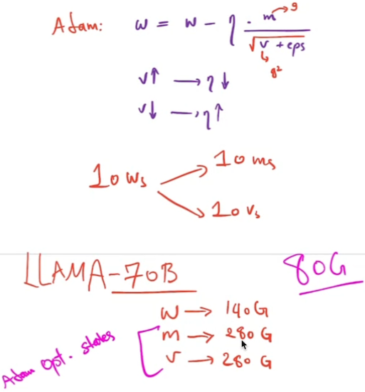
   \[ w_{t+1} = w_t – \alpha \frac{\hat{m}_t}{\sqrt{\hat{v}_t} + \epsilon} \]
   Here, \( \alpha \) is the learning rate, and \( \epsilon \) is a small constant to prevent division by zero.

Detailed Explanation of Benefits

• Adaptive Learning Rates: Each parameter has its own learning rate that adapts based on the gradient history. This means parameters with large gradients will have their learning rates decreased, preventing overshooting, while parameters with small gradients will have their learning rates increased, accelerating convergence.
• Bias Correction: The bias correction ensures that the estimates of the first and second moments are accurate, even in the initial steps. Without bias correction, the moment estimates would be underestimated, leading to suboptimal updates.
• Efficiency and Stability: By adapting the learning rates for each parameter individually, Adam achieves both efficient and stable convergence. It combines the benefits of AdaGrad (handling sparse data well) and RMSProp (dealing with non-stationary objectives).

Example Scenario

Imagine you are training a deep neural network where some parameters require very fine-tuned adjustments (small gradients) while others require larger adjustments (large gradients). A fixed learning rate would be suboptimal:

• Small Gradients: If the learning rate is too low, parameters with small gradients will take a long time to converge.
• Large Gradients: If the learning rate is too high, parameters with large gradients might overshoot and destabilize the training process.

Adam, by adjusting the learning rates based on the first and second moments of the gradients, ensures that each parameter is updated appropriately:

• Parameters with small gradients get a relatively higher learning rate, speeding up their convergence.
• Parameters with large gradients get a relatively lower learning rate, preventing overshooting and ensuring stability.

The first and second moments help adaptive learning rate algorithms like Adam to make more informed, efficient, and stable updates to the model parameters, leading to better and faster convergence.

Weight Decay in Adam vs. AdamW

Weight decay is a regularization technique used to prevent overfitting by penalizing large weights in a model. In the context of the Adam and AdamW optimizers, weight decay is implemented differently, impacting how regularization is applied during the training process. Let’s explore these differences in detail.

Adam with Weight Decay

In the traditional Adam optimizer, weight decay is typically implemented as an L2 regularization term added to the loss function. This approach indirectly influences the parameter updates. The loss function \( L \) with weight decay (L2 regularization) can be written as:

\[ L_{\text{reg}} = L + \frac{\lambda}{2} |w|^2 \]

where \( \lambda \) is the weight decay coefficient, and \( |w|^2 \) is the L2 norm of the weights.

Update Rule for Adam with Weight Decay

Incorporating weight decay in the Adam optimizer involves modifying the gradients as follows:

1. Compute the gradient of the loss function:

\[ \nabla L(w_t) \]

2. Add the weight decay term to the gradient:

\[ g_t = \nabla L(w_t) + \lambda w_t \]

3. Update biased first moment estimate:

\[ m_{t+1} = \beta_1 m_t + (1 – w_1) g_t \]

4. Update biased second moment estimate:

\[ v_{t+1} = \beta_2 v_t + (1 – \beta_2) g_t^2 \]

5. Correct bias in moment estimates:

\[ \hat{m}_{t+1} = \frac{m_{t+1}}{1 – \beta_1^{t+1}} \]

\[ \hat{v}_{t+1} = \frac{v_{t+1}}{1 – \beta_2^{t+1}} \]

6. Update parameters:

\[ w_{t+1} = w_t – \alpha \frac{\hat{m}_{t+1}}{\sqrt{\hat{v}_{t+1}} + \epsilon} \]

AdamW (Decoupled Weight Decay)

AdamW, proposed by Loshchilov and Hutter in their paper “Decoupled Weight Decay Regularization,” decouples the weight decay from the gradient update step. Instead of adding the weight decay term to the gradient, AdamW applies weight decay directly to the weights during the parameter update step.

Update Rule for AdamW

1. Compute the gradient of the loss function:

\[ \nabla L(w_t) \]

2. Update biased first moment estimate:

\[ m_{t+1} = \beta_1 m_t + (1 – \beta_1) g_t \]

3. Update biased second moment estimate:

\[ v_{t+1} = \beta_2 v_t + (1 – \beta_2) g_t^2 \]

4. Correct bias in moment estimates:

\[ \hat{m}_{t+1} = \frac{m_{t+1}}{1 – \beta_1^{t+1}} \]

\[ \hat{v}_{t+1} = \frac{v_{t+1}}{1 – \beta_2^{t+1}} \]

5. Apply weight decay directly to the parameters:

\[ w_{t+1} = w_t – \alpha \frac{\hat{m}_{t+1}}{\sqrt{\hat{v}_{t+1}} + \epsilon} – \alpha \lambda w_t \]

Key Differences

Integration with Gradient Update:

• Adam with Weight Decay: Weight decay is added to the gradient before computing the moment estimates, making weight decay part of the gradient update step.
• AdamW: Weight decay is applied directly to the weights after the gradient-based update step, decoupling the regularization term from the adaptive gradient update.

Impact on Moment Estimates:

• Adam with Weight Decay: The gradient used for updating the moment estimates includes the weight decay term. This means that the moment estimates \( m_t \) and \( v_t \) are influenced by both the loss gradient and the weight decay.
• AdamW: The moment estimates are computed based only on the loss gradient. The weight decay is applied separately, ensuring that the adaptive nature of Adam is not affected by the regularization term.

Hyperparameter Sensitivity:

• Adam with Weight Decay: The effective learning rate can be affected by the weight decay term, as it influences the gradient magnitude.
• AdamW: The learning rate and weight decay are more decoupled, providing more flexibility in tuning these hyperparameters independently.

LARS (Layer-wise Adaptive Rate Scaling)

Problem Addressed

LARS (Layer-wise Adaptive Rate Scaling) is designed to address the issues that arise when training very large deep neural networks, particularly those with millions or billions of parameters. The main problems include:

• Vanishing/Exploding Gradients: In very deep networks, gradients can become extremely small or large, making training unstable or slow.
• Different Magnitudes of Updates: Different layers in a deep network might require different magnitudes of updates. For instance, early layers may need smaller updates compared to later layers due to their differing roles and magnitudes of their weights.

Key Idea

LARS scales the learning rate for each layer individually based on the norm of the weights and the norm of the gradients for that layer. The primary idea is to ensure that the learning rate is appropriately adapted for each layer, preventing some layers from updating too slowly or too quickly.

Update Rule

The learning rate for each layer \( l \) is scaled as follows:

\[ \eta_l = \eta \cdot \frac{| w_l |}{| \nabla L(w_l) | + \epsilon} \]

Here:

• \( \eta \) is the global learning rate.
• \( w_l \) are the weights of layer \( l \).
• \( \nabla L(w_l) \) is the gradient of the loss with respect to \( w_l \).
• \( \epsilon \) is a small constant to prevent division by zero.

The weights are then updated using the scaled learning rate:

\[ w_{l,t+1} = w_{l,t} – \eta_l \cdot \nabla L(w_l) \]

LAMB (Layer-wise Adaptive Moments optimizer for Batch training)

Problem Addressed

LAMB (Layer-wise Adaptive Moments optimizer for Batch training) is an extension of the Adam optimizer designed to work well with large-batch training, which is crucial for speeding up the training process of very large models. The key problems addressed include:

• Training Stability with Large Batches: When using very large batch sizes, training can become unstable. The learning rates need to be carefully adjusted to maintain stability.
• Generalization Performance: Large-batch training can negatively impact the generalization performance of the model.

Key Idea

LAMB combines the adaptive moment estimation from Adam with layer-wise scaling similar to LARS. The idea is to adapt the learning rate for each parameter based on both the layer-wise scaling and the gradient history, ensuring stable and efficient updates even with large batch sizes.

Update Rule

LAMB modifies the Adam update rule by introducing a layer-wise scaling factor. The update steps are:

1. Compute Adam-style moments:
   \[ m_t = \beta_1 m_{t-1} + (1 – \beta_1) \nabla L(w_t) \]
   \[ v_t = \beta_2 v_{t-1} + (1 – \beta_2) (\nabla L(w_t))^2 \]
2. Compute bias-corrected moments:
   \[ \hat{m}_t = \frac{m_t}{1 – \beta_1^t} \]
   \[ \hat{v}_t = \frac{v_t}{1 – \beta_2^t} \]
3. Compute Adam update step:
   \[ r_t = \frac{\hat{m}_t}{\sqrt{\hat{v}_t} + \epsilon} \]
4. Layer-wise scaling factor:
   \[ \eta_t = \eta \cdot \frac{| w_t |}{| r_t |} \]
5. Update weights:
   \[ w_{t+1} = w_t – \eta_t \cdot r_t \]

Here:

• \( \eta \) is the global learning rate.
• \( \epsilon \) is a small constant to prevent division by zero.

Both LARS and LAMB aim to enhance the training of large-scale deep neural networks by adapting the learning rate more intelligently, thereby improving training stability and efficiency.

Gradient Accumulation

Problem Addressed:

Gradient accumulation is a technique used to address the limitations related to memory constraints when training large deep neural networks with high batch sizes. Training with larger batch sizes often leads to more stable updates and faster convergence, but it requires significant GPU memory. When the available GPU memory is insufficient to handle large batches, gradient accumulation allows simulating larger batch sizes by accumulating gradients over multiple smaller batches.

Key Problems Solved:

1. Memory Constraints: Large batch sizes require more memory, which may exceed the capacity of the GPU.
2. Training Stability: Larger batch sizes can lead to more stable and reliable gradient estimates.
3. Effective Learning Rate: By simulating a larger batch size, the effective learning rate can be increased, which may lead to faster convergence.

How Gradient Accumulation Works:

1. Accumulate Gradients: Instead of updating the model parameters after each mini-batch, gradients are accumulated over several mini-batches.
2. Update Parameters: After a specified number of mini-batches (equivalent to the desired large batch size), the accumulated gradients are used to update the model parameters.

Implementation in PyTorch

In PyTorch, gradient accumulation can be implemented by controlling the backward pass and optimizer step manually. Here’s a step-by-step guide on how to do this:

1. Define Accumulation Steps: Decide on the number of mini-batches to accumulate gradients over (let’s call this accumulation_steps).
2. Initialize the Model and Optimizer: Set up your model, loss function, and optimizer as usual.
3. Training Loop: Modify the training loop to accumulate gradients and update the model parameters after the specified number of mini-batches.

import torch
from torch import nn, optim

# Example model, loss function, and optimizer
model = nn.Sequential(nn.Linear(10, 10), nn.ReLU(), nn.Linear(10, 1))
loss_fn = nn.MSELoss()
optimizer = optim.Adam(model.parameters(), lr=0.001)

# Number of accumulation steps
accumulation_steps = 4

# Training loop
for epoch in range(num_epochs):
    for i, (inputs, targets) in enumerate(dataloader):
        # Forward pass
        outputs = model(inputs)
        loss = loss_fn(outputs, targets)

        # Backward pass
        loss.backward()

        # Gradient accumulation: Update parameters every 'accumulation_steps' mini-batches
        if (i + 1) % accumulation_steps == 0:
            optimizer.step()
            optimizer.zero_grad()

# Handle the remaining mini-batches if not divisible by 'accumulation_steps'
if (i + 1) % accumulation_steps != 0:
    optimizer.step()
    optimizer.zero_grad()

Detailed Steps

1. Forward Pass: Compute the output of the model and the loss for each mini-batch.
2. Backward Pass: Call loss.backward() to compute the gradients. These gradients are accumulated in the model parameters.
3. Gradient Accumulation: After accumulation_steps mini-batches, perform an optimization step with optimizer.step() and reset the gradients with optimizer.zero_grad().
4. Handling Remainder: If the total number of mini-batches is not divisible by accumulation_steps, ensure to update the parameters with the remaining gradients.

Benefits of Gradient Accumulation

1. Reduced Memory Usage: By using smaller mini-batches and accumulating gradients, the memory footprint is reduced, making it feasible to train large models on memory-constrained hardware.
2. Improved Stability: Larger effective batch sizes lead to more stable and reliable gradient updates.
3. Flexibility: Allows for training with effectively larger batch sizes without needing additional memory.

Considerations

1. Learning Rate Adjustment: When using gradient accumulation, you may need to adjust the learning rate. Since the effective batch size is larger, the learning rate may need to be scaled appropriately.
2. Accumulation Steps: Choosing the right number of accumulation steps is important. Too few may not provide the desired memory reduction, and too many may slow down the training process.

By leveraging gradient accumulation, you can train deep neural networks with large effective batch sizes even when hardware memory is limited, leading to more stable and potentially faster training.

Activation or Gradient Checkpointing

Problem Addressed:

Activation or gradient checkpointing is a technique designed to address the issue of high memory usage during the training of deep neural networks. Training very deep models requires storing a large number of activations (intermediate outputs of the layers) in memory for the backward pass. This can quickly exceed the available memory, especially on GPUs.

Key Problems Solved:

1. Memory Constraints: Reduces the memory footprint by selectively storing and recomputing activations, allowing the training of deeper models on hardware with limited memory.
2. Scalability: Enables training of very deep neural networks by optimizing the trade-off between memory usage and computational overhead.

How Activation Checkpointing Works

The basic idea behind activation checkpointing is to save memory by not storing all intermediate activations during the forward pass. Instead, only a subset of activations (checkpoints) is stored, and the others are recomputed during the backward pass as needed. This reduces memory usage at the cost of additional computation.

1. Forward Pass: During the forward pass, only the selected checkpoints are stored. The other activations are discarded and need to be recomputed during the backward pass.
2. Backward Pass: When computing gradients, the discarded activations are recomputed from the nearest checkpoint. This allows the backpropagation to proceed as if all activations were stored, but with reduced memory usage.

Implementation in PyTorch

PyTorch provides utilities to implement activation checkpointing. Here’s a basic example:

1. Import Checkpoint Function: Use the checkpoint function from torch.utils.checkpoint.
2. Wrap the Model: Wrap parts of the model in a checkpoint to control which activations to store and which to recompute.

import torch
import torch.nn as nn
import torch.optim as optim
from torch.utils.checkpoint import checkpoint

# Define a simple model with checkpoints
class CheckpointedModel(nn.Module):
    def __init__(self):
        super(CheckpointedModel, self).__init__()
        self.layer1 = nn.Linear(10, 50)
        self.layer2 = nn.Linear(50, 50)
        self.layer3 = nn.Linear(50, 10)

    def forward(self, x):
        x = checkpoint(self.layer1, x)
        x = checkpoint(self.layer2, x)
        x = self.layer3(x)
        return x

# Initialize model, loss function, and optimizer
model = CheckpointedModel()
loss_fn = nn.MSELoss()
optimizer = optim.Adam(model.parameters(), lr=0.001)

# Training loop
for epoch in range(num_epochs):
    for inputs, targets in dataloader:
        # Forward pass
        outputs = model(inputs)
        loss = loss_fn(outputs, targets)

        # Backward pass
        optimizer.zero_grad()
        loss.backward()
        optimizer.step()

Benefits of Activation Checkpointing

1. Memory Efficiency: Significantly reduces the memory required to store activations, allowing training of larger and deeper models on limited hardware.
2. Scalability: Enables scaling up model size and depth without hitting memory limits, facilitating more complex and capable neural networks.
3. Flexibility: Provides control over the memory-computation trade-off, allowing tuning based on the specific hardware and model requirements.

Considerations

1. Increased Computation: Activation checkpointing introduces additional computation during the backward pass due to recomputing activations. This can lead to longer training times.
2. Checkpoint Selection: Careful selection of checkpoints is important to balance memory savings and computational overhead. Too few checkpoints can lead to high recomputation costs, while too many may not save much memory.
3. Implementation Complexity: Requires modifications to the model code to implement checkpointing, adding some complexity to the training loop.

Example Scenario

Consider training a deep neural network with many layers on a GPU with limited memory:

• Without Checkpointing: All activations are stored during the forward pass, leading to high memory usage and potentially running out of memory.
• With Checkpointing: Only selected activations are stored, and others are recomputed during the backward pass. This reduces memory usage, allowing the model to fit into the GPU memory. The trade-off is additional computation during the backward pass, but the training process becomes feasible.

References

1. Kingma, D. P., & Ba, J. (2014). Adam: A Method for Stochastic Optimization. arXiv preprint arXiv:1412.6980. Retrieved from https://arxiv.org/abs/1412.6980
2. Loshchilov, I., & Hutter, F. (2017). Decoupled Weight Decay Regularization. arXiv preprint arXiv:1711.05101. Retrieved from https://arxiv.org/abs/1711.05101
3. You, Y., Gitman, I., & Ginsburg, B. (2017). Large Batch Training of Convolutional Networks. arXiv preprint arXiv:1708.03888. Retrieved from https://arxiv.org/abs/1708.03888
4. You, Y., Li, J., Reddi, S., Hseu, J., Kumar, S., Bhojanapalli, S., Song, X., Demmel, J., Keutzer, K., & Hsieh, C.-J. (2019). Large Batch Optimization for Deep Learning: Training BERT in 76 minutes. arXiv preprint arXiv:1904.00962. Retrieved from https://arxiv.org/abs/1904.00962
5. Distill. (2017). Visualizing and Understanding Momentum. Distill. Retrieved from https://distill.pub/2017/momentum/
6. Lightly AI. (n.d.). Which Optimizer Should I Use for My Machine Learning Project? Lightly AI Blog. Retrieved from https://www.lightly.ai/post/which-optimizer-should-i-use-for-my-machine-learning-project