Introduction

In our last discussion, we explored dropout regularization techniques, which involve randomly setting a fraction of the activations to zero during training. This helps prevent overfitting by encouraging the network to learn redundant representations and improving generalization.

Today, we will extend our focus to other regularization methods, including L1 and L2 regularization, label smoothing, CutMix, and MixUp. Additionally, we will discuss the use of Monte Carlo Dropout during inference to evaluate model confidence.

The Challenge of Model Generalization

Overfitting occurs when a neural network learns the training data too well, including its noise and outliers. This leads to a model that performs exceptionally on training data but poorly on unseen test data because it has not generalized well.

The primary negative impact of overfitting is reduced model performance on new, unseen data. An overfitted model captures the noise in the training data as if it were a true signal, leading to poor predictions and decreased reliability in practical applications.

Regularization techniques introduce additional constraints or penalties to the model to prevent it from fitting the training data too closely. By doing so, regularization helps improve the model’s generalization capabilities, ensuring better performance on new data.

L1 and L2 Regularizations

L1 Regularization:

Impact on Weight Magnitude and Feature Selection

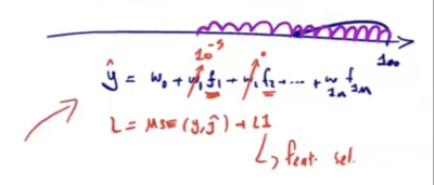
L1 regularization adds a penalty proportional to the absolute value of the weights. This encourages the network to drive some weights to exactly zero, effectively performing feature selection by eliminating irrelevant or less important features. As a result, the model becomes sparse and focuses only on the most significant features.

The L1 regularization term is expressed as:

\[ L1_{\text{reg}} = \lambda \sum_{i} |w_i| \]

where \(\lambda\) is the regularization strength (a hyperparameter) and \(w_i\) are the model weights.

L2 Regularization (Weight Decay):

Impact on Weight Magnitude and Model Generalization

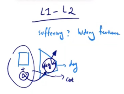
L2 regularization reduces the magnitude of less important weights without typically setting them to zero. By minimizing reliance on these less critical features, the model becomes less dependent on them, effectively “hiding” these features from the network. This balanced approach contributes to improved model stability and resilience, making it more effective in handling diverse and unseen data.

The L2 regularization term is expressed as:

\[ L2_{\text{reg}} = \lambda \sum_{i} w_i^2 \]

where \(\lambda\) is the regularization strength (a hyperparameter) and \(w_i\) are the model weights. The total loss function becomes:

\[ Loss_{total} = Loss_{original} + L2_{reg} \]

Use in CNNs to Prevent Overfitting

L2 regularization, often referred to as weight decay, is commonly used in CNNs to prevent overfitting. It ensures that the learned filters (weights) are not too sensitive to the training data, improving the model’s generalization.

Why Smaller Weights Matter in Neural Networks?

One of the key principles in neural networks is to prevent them from relying heavily on any single piece of information. By “hiding” or reducing the importance of less critical features, regularization techniques force the network to perform more effectively with fewer resources, enhancing its ability to generalize and find optimal solutions.

In general, it is preferable to have a network with smaller weights rather than large ones. Let’s consider an example to illustrate why this is important.

Imagine we have an image of a dog, and our neural network correctly identifies it as a dog. The image contains numerous pixel values, each contributing to the final prediction. If we slightly alter this image by increasing the intensity of all pixels by a small value, say 2 units, this change is almost imperceptible to the human eye. However, when we feed this modified image back into the network, a network with large weights might misclassify it as a cat.

This misclassification happens because the small change in pixel values gets amplified by the large weights. After the multiplication, the small delta becomes a significant value, affecting the network’s decision. Therefore, a network with large weights is highly sensitive to trivial changes in the input, which is undesirable. Ideally, we want the network to provide consistent predictions even with slight variations in the input.

Robust and Generalizable Networks

Networks with smaller weights are more robust and generalizable. They are less sensitive to minor changes in the input, ensuring consistent and reliable predictions. L1 and L2 regularization techniques were proposed to achieve this by penalizing large weights and promoting smaller, more stable ones.

Regularization in the Loss Function

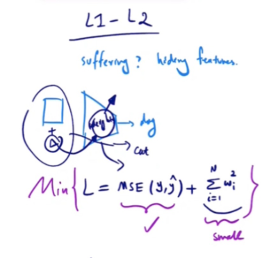
Let us examine the loss function with an L2 regularization term. For simplicity, we’ll consider the Mean Squared Error \(MSE\) loss with L2 regularization:

\[ L = \text{MSE}(y, \hat{y}) + \lambda \sum_{i} w_i^2 \]

In this equation:

• \(\text{MSE}(y, \hat{y})\) is the original loss function.
• \(\lambda \sum_{i} w_i^2\) is the L2 regularization term.
• \(\lambda\) is the regularization strength.
• \(w_i\) are the model weights.

When the weights are large, the regularization term also becomes large, increasing the total loss. The optimization process aims to minimize this loss, which in turn ensures that the weights are kept small.

Weight Updates in the Optimizer

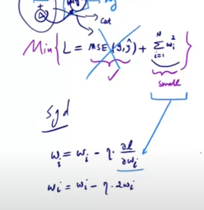
Let’s consider how weights are updated using the Stochastic Gradient Descent \(SGD\) optimizer. In general, SGD updates the weight values as follows:

\[ w_i = w_i – \eta \frac{\partial L}{\partial w_i} \]

where:

• \(w_i\) is the weight.
• \(\eta\) is the learning rate.
• \(\frac{\partial L}{\partial w_i}\) is the gradient \(partial derivative\) of the loss with respect to the weight.

L2 Regularization Impact on Weight Updates

Including the L2 regularization term, the update rule becomes:

\[ w_i = w_i – \eta \left( \frac{\partial \text{MSE}}{\partial w_i} + 2\lambda w_i \right) \]

This update rule ensures that large weights are penalized, effectively reducing their values over time and promoting smaller, more stable weights.

To understand the impact of L2 regularization on weight updates, let’s consider the following simplified scenario:

1. Assume that x-axis represents \(w_i\), the weight.
2. The initial value of \(w_i\) is 1.
3. The learning rate \(\eta\) is 0.1.
4. We’ll use only the L2 regularization term and ignore the MSE term for this explanation.

The L2 regularization term in the loss function is:

\[ L2_{\text{reg}} = \lambda \sum_{i} w_i^2 \]

For simplicity, we will temporarily ignore the regularization strength term, \(\lambda\). Therefore, the gradient of the L2 regularization term with respect to \(w_i\) is:

\[ \frac{\partial L2_{\text{reg}}}{\partial w_i} = 2w_i \]

Using Stochastic Gradient Descent \(SGD\) for weight updates, the update rule for \(w_i\) is:

\[ w_i = w_i – \eta \cdot \frac{\partial L2_{\text{reg}}}{\partial w_i} \]

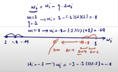
\[ w_i = w_i – \eta \cdot 2 \cdot w_i \]

Continuous Weight Update with L2 Regularization

When applying L2 regularization, each weight update reduces the value of \(w_i\)​, causing it to approach zero over time. This happens because L2 regularization penalizes larger weights. Additionally, the change \(delta\) in \(w_i\) decreases with each update, indicating diminishing adjustments as weights get smaller. L2 regularization affects both positive and negative weights by reducing their magnitudes, promoting a balanced and distributed set of weights. This helps achieve a more stable and generalizable model, preventing overfitting and enhancing robustness to small input variations.

Step-by-Step Example with L2 Regularization

Step-by-Step Example (Positive)

1. Initial Weight Update (from 1 to 0.8):

• Initial \( w_i = 1 \)
• Learning rate \( \eta = 0.1 \)
• Gradient: \( \nabla_{w_i} = 2 \times 1 = 2 \)
• Update: \( w_i = 1 – 0.1 \times 2 = 1 – 0.2 = 0.8 \)
• Delta: \( 1 – 0.8 = 0.2 \)

2. Second Weight Update (from 0.8 to 0.64):

• New \( w_i = 0.8 \)
• Gradient: \( \nabla_{w_i} = 2 \times 0.8 = 1.6 \)
• Update: \( w_i = 0.8 – 0.1 \times 1.6 = 0.8 – 0.16 = 0.64 \)
• Delta: \( 0.8 – 0.64 = 0.16 \)

Step-by-Step Example (Negative)

1. Initial Weight Update (from -1 to -0.8):

• Initial \( w_i = -1 \)
• Learning rate \( \eta = 0.1 \)
• Gradient: \( \nabla_{w_i} = 2 \times (-1) = -2 \)
• Update: \( w_i = -1 – 0.1 \times (-2) = -1 + 0.2 = -0.8 \)
• Delta: \( -0.8 – (-1) = 0.2 \)

2. Second Weight Update (from -0.8 to -0.64):

• New \( w_i = -0.8 \)
• Gradient: \( \nabla_{w_i} = 2 \times (-0.8) = -1.6 \)
• Update: \( w_i = -0.8 – 0.1 \times (-1.6) = -0.8 + 0.16 = -0.64 \)
• Delta: \( -0.64 – (-0.8) = 0.16 \)

Observations

1. Weight Decay: With each update, the weight value \( w_i \) gets smaller in magnitude. For positive weights, \( w_i \) decreased from 1 to 0.8, and then from 0.8 to 0.64. Similarly, for negative weights, \( w_i \) increased from -1 to -0.8, and then from -0.8 to -0.64.
2. Diminishing Delta: The change \(delta\) in \( w_i \) gets smaller with each step. For positive weights, the delta decreased from 0.2 to 0.16. For negative weights, the delta also decreased from 0.2 to 0.16.
3. Symmetrical Effect: L2 regularization affects both positive and negative weights symmetrically, reducing their magnitudes over time. This helps in achieving smaller, more stable weights, promoting a balanced and distributed set of weights that enhances model generalization and prevents overfitting.

Weight Decay and the Balance of Forces

Notice how weights decay even in the absence of the actual loss function. If you apply L2 regularization without the loss function, the regularization term alone would drive all weights to zero. This is because the regularization term penalizes large weights, and minimizing it would result in weights approaching zero.

However, in practice, we always have the loss function present alongside the regularization term. This introduces a dynamic interaction—a “battle”—between the loss function and the regularization term:

• Regularization Term: Aims to reduce weights to zero to minimize the regularization penalty.
• Loss Function: Seeks to adjust weights to minimize the prediction error, which often requires non-zero weights.

The Battle and the Sweet Spot

The optimal solution for the regularization term alone would be to make all weights zero, which would result in no predictive power and thus a very high loss. On the other hand, the loss function by itself would adjust weights solely to minimize prediction error, potentially leading to overfitting with large weights.

This interplay results in a balancing act:

• The network increases weights to solve the problem posed by the loss function, improving its predictions.
• The regularization term pulls weights towards zero to prevent overfitting, promoting generalization.

This continuous battle between the loss function and the regularization term leads to an equilibrium, where the weights are adjusted to a point that neither function dominates completely. This equilibrium represents the “sweet spot,” where the model achieves a good balance between fitting the training data and maintaining generalization to unseen data.

The Nature of L2 Regularization

L2 regularization tends to reduce the weights of a model, pushing them very close to zero but not exactly zero. The decay of the weights is determined by the term \( \eta \cdot \frac{\partial L2_{\text{reg}}}{\partial w_i} \). In the example discussed, this decay is specifically \( 2 \cdot w_i \). The change in weight \((\Delta w_i)\) is directly influenced by the value of \( w_i \). When the weights are large, the changes will be more significant but will still decrease as they approach zero. Conversely, as \( w_i \) approaches zero, the change in weight also diminishes.

Loss Function with L1 Regularization

The loss function with L1 regularization is given by:

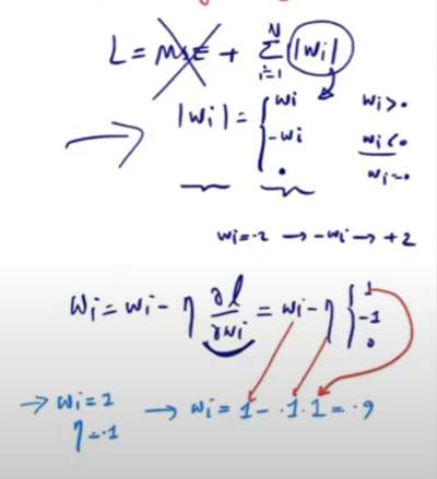
\[ L = \text{MSE}(y, \hat{y}) + \lambda \sum_{i} |w_i| \]

Where:

• \( \text{MSE}(y, \hat{y}) \) is the Mean Squared Error between the true values \( y \) and the predicted values \( \hat{y} \).
• \( \lambda \sum_{i} |w_i| \) is the L1 regularization term.
• \( \lambda \) is the regularization strength.
• \( w_i \) are the model weights.

Absolute Value of \( w_i \)

The absolute value function for \( w_i \) is defined as:

\[ |w_i| =
\begin{cases}
-w_i & \text{if } w_i < 0 \\
w_i & \text{if } w_i > 0 \\
0 & \text{if } w_i = 0
\end{cases}
\]

Derivative of Loss with Respect to \( w_i \)

The derivative of \( L \) with respect to \( w_i \) depends on the sign of \( w_i \):

\[
\frac{\partial L}{\partial w_i} =
\begin{cases}
\frac{\partial \text{MSE}(y, \hat{y})}{\partial w_i} + \lambda & \text{if } w_i > 0 \\
\frac{\partial \text{MSE}(y, \hat{y})}{\partial w_i} – \lambda & \text{if } w_i < 0 \\
\frac{\partial \text{MSE}(y, \hat{y})}{\partial w_i} & \text{if } w_i = 0
\end{cases}
\]

Where:

• \( \text{sign}(w_i) \) is the sign function that returns:
• \( 1 \) if \( w_i \) is positive.
• \( -1 \) if \( w_i \) is negative.
• \( 0 \) if \( w_i \) is zero.

Weight Update Using Stochastic Gradient Descent (SGD)

The general update rule for weights using SGD is:

\[ w_i = w_i – \eta \frac{\partial L}{\partial w_i} \]

For simplicity, we will temporarily ignore MSE term’s derivative \( \frac{\partial \text{MSE}(y, \hat{y})}{\partial w_i} \) and the regularization strength term \( \lambda \). Therefore, the gradient of the L1 regularization term with respect to \( w_i \) is:

\[ \frac{\partial}{\partial w_i} \left( |w_i| \right) =

\begin{cases}

1 & \text{if } w_i > 0 \\

-1 & \text{if } w_i < 0 \\

0 & \text{if } w_i = 0

\end{cases}

\]

Step-by-Step Example with L1 Regularization

Step-by-Step Example (Positive)

1. Initial Weight Update (from 1 to 0.9):

• Initial \( w_i = 1 \)
• Learning rate \( \eta = 0.1 \)
• Gradient: \( \nabla_{w_i} = 1 \)
• Update: \( w_i = 1 – 0.1 \times 1 = 0.9 \)
• Delta: \( 1 – 0.9 = 0.1 \)

2. Second Weight Update (from 0.9 to 0.8):

• New \( w_i = 0.9 \)
• Gradient: \( \nabla_{w_i} = 1 \)
• Update: \( w_i = 0.9 – 0.1 \times 1 = 0.8 \)
• Delta: \( 0.9 – 0.8 = 0.1 \)

Step-by-Step Example (Negative)

1. Initial Weight Update (from -1 to -0.9):

• Initial \( w_i = -1 \)
• Learning rate \( \eta = 0.1 \)
• Gradient: \( \nabla_{w_i} = -1 \)
• Update: \( w_i = -1 – 0.1 \times (-1) = -0.9 \)
• Delta: \( -0.9 – (-1) = 0.1 \)

2. Second Weight Update (from -0.9 to -0.8):

• New \( w_i = -0.9 \)
• Gradient: \( \nabla_{w_i} = -1 \)
• Update: \( w_i = -0.9 – 0.1 \times (-1) = -0.8 \)
• Delta: \( -0.8 – (-0.9) = 0.1 \)

Observations

1. Weight Decay: With each update, the weight value \( w_i \) gets smaller in magnitude. For positive weights, \( w_i \) decreased from 1 to 0.9, and then from 0.9 to 0.8. Similarly, for negative weights, \( w_i \) increased from -1 to -0.9, and then from -0.9 to -0.8.
2. Constant Delta: The change \(delta\) in \( w_i \) remains constant with each step. For both positive and negative weights, the delta was consistently 0.1 with each update.
3. Symmetrical Effect: L1 regularization affects both positive and negative weights symmetrically, reducing their magnitudes by a constant factor during each update. This promotes sparsity in the model weights, encouraging many weights to become exactly zero.

Label Smoothing in CNN

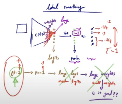
In a Convolutional Neural Network (CNN) designed to classify images of dogs into five distinct breeds, the process involves several crucial steps. When an image is input into the model, it undergoes various convolutional and pooling layers that extract and refine features. The final layer of the network outputs a set of raw values (unnormalized log probabilities) known as \(logits\), which correspond to the five possible breeds.

Classification Process and Cross-Entropy Loss

These logits are then passed through a softmax layer, a crucial component that converts (normalizes) them into a probability distribution. The softmax function transforms the logits into probabilities that sum to 1, representing the model’s confidence in each breed classification. For example, if the logits output by the model are \([1.0, 2.5, 1.0, 0.5, 0.0]\), the softmax function will process these values and output probabilities like \([0.14, 0.57, 0.14, 0.09, 0.06]\). These probabilities indicate the model’s certainty that the input image belongs to each respective breed.

To determine the accuracy of the model, these predicted probabilities are compared against the ground truth labels, which are typically represented as one-hot encoded vectors. A one-hot encoded vector is a binary vector used to indicate the correct class in a classification problem. For instance, if a dog belongs to the second breed, the corresponding one-hot encoded vector would be \([0, 1, 0, 0, 0]\). This vector has a ‘1’ in the position of the correct class (second breed) and ‘0’s elsewhere.

The cross-entropy loss function is used to measure the difference between the predicted probabilities and the one-hot encoded ground truth. The loss for a single example is calculated as:

\[
\text{Loss} = – \sum (y_i \cdot \log(p_i))
\]

where \(y_i\) is the ground truth probability for class \( i \), and \(p_i\) is the predicted probability for class \( i \). The goal is to minimize this loss, making the predicted probabilities as close as possible to the one-hot vector, with the probability for the correct class close to 1 and the probabilities for other classes close to 0.

The Challenge with Large Weights

Achieving a probability of 1 for the correct class requires the input logit for that class to be significantly larger than the logits for other classes. For example, consider the logits \([-1.2, 3.5, 0.2, -0.9, -1.5]\) for five classes. After applying softmax, the probabilities might be \([0.01, 0.94, 0.02, 0.02, 0.01]\). The second class has a high probability because its logit \(3.5\) is much larger than the others.

However, achieving a probability close to 1 necessitates very large weights, which can lead to overfitting and poor generalization.

Introducing Label Smoothing

Label smoothing, a regularization technique introduced in the Inception-v3 architecture (Szegedy et al., 2016), addresses this issue. Instead of aiming for a probability of 1 for the ground truth, label smoothing relaxes this requirement slightly. For instance, the ground truth value might be set to 0.9 instead of 1. This means the network only needs to produce a probability of 0.9 for the correct class, requiring smaller logits and thus smaller weights.

Determining Smoothed Labels

The values for smoothed labels are determined by a parameter known as the smoothing factor, typically denoted as \(\alpha\). This factor is chosen before training and is a hyperparameter that can be tuned. For a given label smoothing factor \(\alpha\), the smoothed labels are computed as follows:

• For the correct class: \(y_{\text{correct}} = 1 – \alpha\)
• For the incorrect classes: \(y_{\text{incorrect}} = \frac{\alpha}{K – 1}\)

where \(K\) is the number of classes.

For example, if \(\alpha = 0.1\) and there are 5 classes \((K = 5)\):

• The smoothed label for the correct class is \(0.9\)
• The smoothed labels for the incorrect classes are \(0.025\)

This results in smoothed labels like \([0.025, 0.9, 0.025, 0.025, 0.025]\).

Concrete Example

Let’s illustrate this with an example. Suppose the original one-hot encoded ground truth for a dog belonging to the second breed is \([0, 1, 0, 0, 0]\). With label smoothing, this might be adjusted to \([0.025, 0.9, 0.025, 0.025, 0.025]\).

Process:

1. Logits Calculation: Assume the network outputs the logits \([1.0, 2.5, 1.0, 0.5, 0.0]\).
2. Softmax Calculation: The softmax function normalizes these logits into probabilities using the following formula:
   \[
   \text{softmax}(z_i) = \frac{e^{z_i}}{\sum_{j} e^{z_j}}
   \] Where \( z_i \) is the logit for the \( i \)-th class and the denominator is the sum of the exponentials of all logits.

• Calculate the exponentials of the logits:
  \[
  e^{1.0} \approx 2.718, \quad e^{2.5} \approx 12.182, \quad e^{1.0} \approx 2.718, \quad e^{0.5} \approx 1.649, \quad e^{0.0} = 1
  \]
• Sum of exponentials:
  \[
  2.718 + 12.182 + 2.718 + 1.649 + 1 = 20.267
  \]
• Calculate the softmax probabilities:
  \[
  \text{softmax}(1.0) = \frac{2.718}{20.267} \approx 0.134
  \]
  \[
  \text{softmax}(2.5) = \frac{12.182}{20.267} \approx 0.601
  \]
  \[
  \text{softmax}(1.0) = \frac{2.718}{20.267} \approx 0.134
  \]
  \[
  \text{softmax}(0.5) = \frac{1.649}{20.267} \approx 0.081
  \]
  \[
  \text{softmax}(0.0) = \frac{1}{20.267} \approx 0.049
  \] So, the probabilities are approximately:
  \[
  [0.134, 0.601, 0.134, 0.081, 0.049]
  \] For ease of explanation and to fit the narrative, we slightly adjusted these values to:
  \[
  [0.14, 0.57, 0.14, 0.09, 0.06]
  \]

3. Cross-Entropy Loss with Smoothing: The cross-entropy loss is calculated using the smoothed labels, comparing the predicted probabilities \([0.14, 0.57, 0.14, 0.09, 0.06]\) to the smoothed labels \([0.025, 0.9, 0.025, 0.025, 0.025]\): \[
   \text{Loss} = – \left( 0.025 \cdot \log(0.14) + 0.9 \cdot \log(0.57) + 0.025 \cdot \log(0.14) + 0.025 \cdot \log(0.09) + 0.025 \cdot \log(0.06) \right)
   \] Calculating each term:
   \[
   0.025 \cdot \log(0.14) \approx 0.025 \cdot (-1.966) = -0.049
   \]
   \[
   0.9 \cdot \log(0.57) \approx 0.9 \cdot (-0.562) = -0.506
   \]
   \[
   0.025 \cdot \log(0.14) \approx 0.025 \cdot (-1.966) = -0.049
   \]
   \[
   0.025 \cdot \log(0.09) \approx 0.025 \cdot (-2.407) = -0.060
   \]
   \[
   0.025 \cdot \log(0.06) \approx 0.025 \cdot (-2.813) = -0.070
   \] Summing these terms:
   \[
   \text{Loss} \approx -(-0.049 – 0.506 – 0.049 – 0.060 – 0.070) = 0.734\]

Cross-Entropy Loss Without Label Smoothing

To provide a comparison, let’s calculate the cross-entropy loss without label smoothing using the one-hot encoded ground truth.

Using the predicted probabilities \([0.14, 0.57, 0.14, 0.09, 0.06]\) and the one-hot encoded ground truth \([0, 1, 0, 0, 0]\), the cross-entropy loss is: \[ \text{Loss} = – \sum_{i} (y_i \cdot \log(p_i)) \]

\[
\text{Loss} = – \left( 0 \cdot \log(0.14) + 1 \cdot \log(0.57) + 0 \cdot \log(0.14) + 0 \cdot \log(0.09) + 0 \cdot \log(0.06) \right)
\]

Since the ground truth is one-hot encoded, it only has a value of 1 for the correct class (second breed) and 0 for the others. Therefore, the loss simplifies to:

\[
\text{Loss} = – \log(0.57) \approx -(-0.562) = 0.562
\]

Analysis of Cross-Entropy Loss with and without Label Smoothing

By comparing the loss values, we observe:

• Without label smoothing: Loss is 0.562
• With label smoothing: Loss is 0.734

Although the immediate loss value with label smoothing initially is higher, label smoothing helps the model to generalize better, leading to improved performance on validation and test sets. This is achieved by preventing the model from becoming overly confident, thereby reducing the risk of overfitting.

Mixup, and Cutmix Data Augmentation Techniques

MixUp

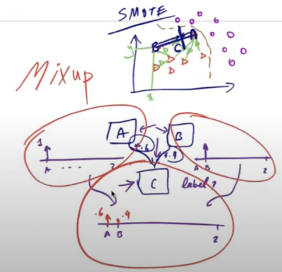
MixUp is an innovative data augmentation technique that blends two images and their corresponding labels to create a new synthetic image and label. Here’s how it works:

1. Image Blending: Given two images, A (dog) and B (cat), a new image C is created by linearly interpolating them:
   \[ C = \lambda A + (1 – \lambda) B \]
   where (\lambda ) is a random number between 0 and 1. This results in an image where features of both A and B are visible, creating a visually ambiguous image.
2. Label Blending: The labels for the new image C are also interpolated. If A’s label is 1, 0 and B’s label is 0, 1, the label for C will be:
   \[ \text{Label}_C = \lambda \cdot \text{Label}_A + (1 – \lambda) \cdot \text{Label}_B \]
   resulting in a soft label, such as [0.6, 0.4], reflecting the mixed nature of the image.

Benefits of MixUp

• Learning Ambiguity: MixUp helps the network learn that real-world data can be ambiguous and that there can be uncertainty in classification. For instance, an image might prominently feature a dog but also have a cat in the background. In such cases, it is unrealistic for the model to predict with 100% certainty that the image contains only a dog.
• Improved Generalization: By training on mixed images and soft labels, the network becomes more robust and generalizes better to unseen data. It learns to make more nuanced predictions rather than being overly confident in its classifications.

Practical Application

In real-world scenarios, like an image with a dog in the foreground and a small cat in the background, MixUp encourages the model to account for the presence of multiple objects and their relative prominence. This results in more accurate and reliable predictions, reflecting the true complexity of the data.

CutMix

CutMix is an advanced data augmentation technique used primarily in image classification and segmentation tasks. Here’s how it works:

1. Image Blending: Given two images, A and B, a new image C is created by cutting a region from image B and pasting it into image A. This creates a composite image that contains features from both A and B.
2. Ground Truth Labels: For image segmentation applications, the corresponding segmentation masks for images A and B are also blended. The mask for the new image C is created by cutting a region from mask B and pasting it into mask A. This ensures that the new image has a consistent segmentation mask.

Benefits of CutMix

• Increased Robustness: By mixing parts of different images, CutMix helps the model learn to recognize objects in varied contexts and increases robustness to occlusions and background variations.
• Improved Generalization: CutMix helps reduce overfitting by providing more diverse training samples, leading to better generalization on unseen data.

Example

1. Creating Image C:

• Cut a rectangular region from image B.
• Paste this region into image A to form a new image C.

2. Creating Mask for C:

• Similarly, cut the corresponding region from mask B.
• Paste this region into mask A to form the new mask for image C.

This technique enhances the training dataset by generating more varied samples, helping the model learn to handle complex and mixed scenarios.

Dropout to Evaluate Model Confidence During Inference

Dropout Overview: Dropout is typically used during training to prevent overfitting by randomly setting a fraction of the input units to zero at each update.

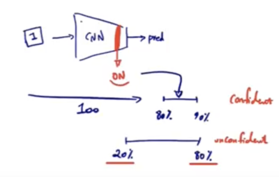
Inference with Dropout: During inference, dropout is usually turned off, but it can be kept on to introduce stochasticity. Each forward pass with dropout generates different predictions due to the randomness of the dropout mask. This technique, known as Monte Carlo Dropout, estimates model uncertainty, providing insights into the confidence of the model’s predictions.

Evaluating Confidence:

1. Multiple Predictions: By performing multiple forward passes (e.g., 100), each with a different dropout mask, we can observe the variability in predictions.
2. Confidence Interval: The range of predicted probabilities can be analyzed. For instance, if the probability of the image being a dog is consistently between 80% and 90% across 100 predictions, this indicates a high confidence level in the model’s prediction.

Detailed Example:

Suppose you have a CNN model that classifies an image as either a dog or a cat. During inference, you apply dropout and perform 100 forward passes with the same input image.

1. High Confidence Scenario:

• You observe that the probability of the image being a dog ranges from 80% to 90%.
• This narrow range indicates the model’s confidence in predicting the image as a dog.
• The model is consistently leaning towards the same class, showing reliability in its prediction.

2. Low Confidence Scenario:

• The probability of the image being a dog ranges widely from 20% to 80%.
• This wide range shows the model’s uncertainty, indicating that it is confused and not confident in its prediction.
• The model’s outputs vary significantly, reflecting ambiguity in distinguishing between the classes.

By applying dropout during inference and analyzing the range of predictions, you can assess the model’s confidence and reliability, identifying when it might be uncertain or confused about its predictions.

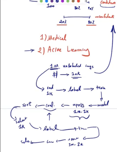
Application in Medical Diagnostics

By leveraging the confidence information extracted using dropout during inference, we can make more informed decisions in critical applications such as medical diagnostics.

Practical Implications:

• Uncertain Diagnoses: If the model shows low confidence (e.g., probabilities ranging widely), it suggests that the model is unsure about its diagnosis.
• Liability Mitigation: In such cases, it might be prudent to withhold the diagnosis from the doctor or patient to avoid potential liabilities and instead flag the case for further review by a human expert.

This approach ensures that only confident predictions are acted upon, improving the reliability and safety of automated decision-making systems.

Application in Active Learning

Active learning is a technique used to maximize the efficiency of labeling data by selecting the most informative samples.

Problem: You have a dataset of 1 million unlabeled images and a budget to label only 1,000 images.

Solution:

1. Initial Labeling: Randomly select 1,000 images, label them, and train the model.
2. Confidence-Based Sampling:

• Apply the model to the remaining (1,000,000 – 1,000) unlabeled images with dropout on to obtain confidence scores.
• Sort the images based on their confidence scores.
• Select the 1,000 images with the lowest confidence (most uncertain predictions) for labeling.

3. Iterative Process:

• Repeat the process of labeling the least confident images and retraining the model.
• Continue for 10 iterations to fit the budget for labeling 10,000 samples.

Importance: Confidence-based sampling helps in selecting the most informative samples that the model is uncertain about, leading to better learning and more efficient use of the labeling budget.

Active learning was a hot topic around 2017 and 2018, with many companies offering labeling services aiming to optimize the labeling process and save costs. Confidence is a crucial metric in active learning, though other metrics can also be considered.

Conclusion

In conclusion, understanding and implementing various regularization techniques is crucial for improving the generalization and robustness of neural networks. Techniques like L1 and L2 regularization, label smoothing, CutMix, and MixUp, each contribute uniquely to preventing overfitting and enhancing model performance on unseen data. Monte Carlo Dropout during inference allows for a deeper assessment of model confidence, which is particularly useful in critical applications such as medical diagnostics and active learning. By leveraging these methods, one can build more reliable and efficient machine learning models.