Enhancing Neural Network Performance with Dropout Techniques
Introduction
In the field of machine learning, neural networks are highly effective, excelling in tasks like image recognition and natural language processing. However, these powerful models often face a significant challenge: overfitting. Overfitting is akin to training a student only with past exam questions – they perform well on those specific questions but struggle with new topics. Similarly, an overfitted neural network performs well on training data but poorly on new, real-world examples.
To tackle overfitting, machine learning experts use various techniques, with dropout being one of the simplest yet most effective methods. Dropout works like a coach who occasionally benches players during practice to promote teamwork and prevent dependence on a few stars. In neural networks, dropout randomly turns off neurons during training, encouraging the network to learn stronger and more independent patterns.
Understanding Dropout
Dropout is a regularization technique that involves randomly deactivating a certain percentage of neurons in a neural network during training. This simple approach significantly enhances the network’s ability to generalize, preventing it from overfitting to the training data.
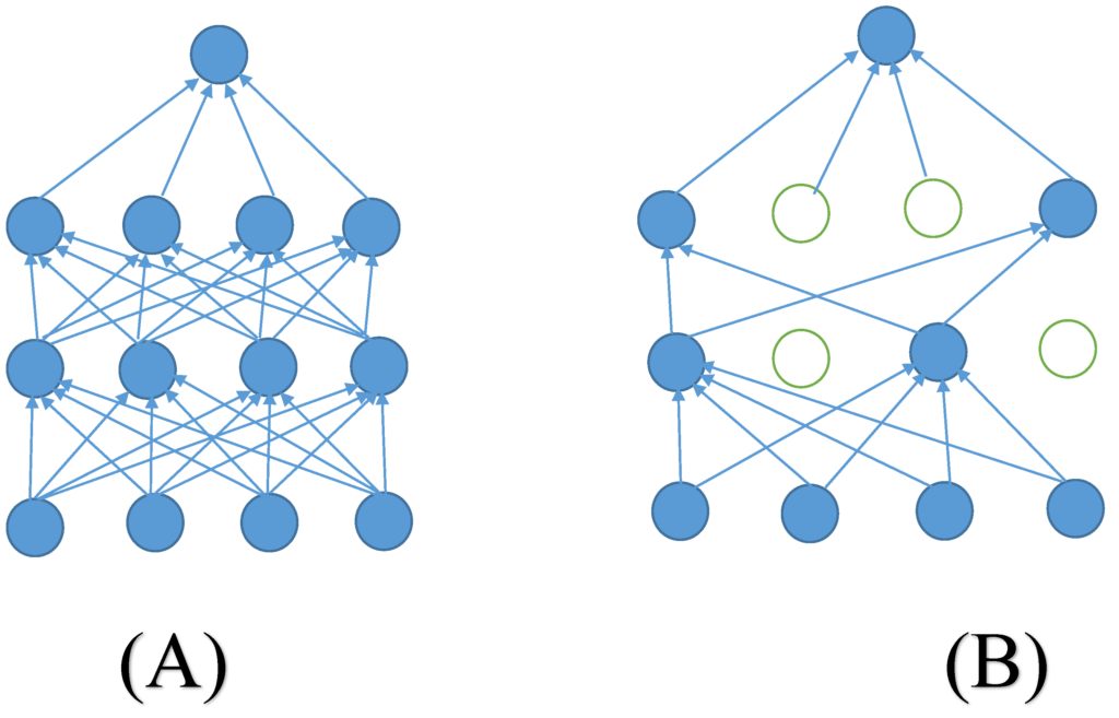
How Dropout Works
Training Phase:
- For each forward pass, a subset of neurons is randomly selected to be dropped out.
- The activations of these neurons are set to zero.
- The remaining neurons compute the network’s output as usual.
- Backpropagation updates the weights of all neurons, including the dropped-out ones.
This process forces the network to learn more robust representations of the data, as it cannot rely on any single neuron or group of neurons. This makes the network more adaptable and less prone to overfitting.
Key Benefits of Dropout
- Prevents Overfitting: Dropout helps prevent the network from memorizing the training data, leading to better generalization on unseen data.
- Improves Model Performance: Dropout often leads to significant improvements in model performance, especially on complex tasks.
- Reduces Training Time: Dropout can sometimes reduce the training time of a neural network.
- Mitigates Vanishing Gradients: Dropout can help reduce the risk of vanishing gradients, which can hinder the training of deep neural networks.
Implementing Dropout from Scratch
In this section, we will implement a neural network with dropout from scratch using NumPy. We’ll train it on the MNIST dataset and compare its performance with a similar network without dropout.
Step 1: Data Preparation
import numpy as np
from sklearn.datasets import fetch_openml
from sklearn.model_selection import train_test_split
from sklearn.preprocessing import OneHotEncoder
import matplotlib.pyplot as plt

def preprocess_data():
    """
    Fetches the MNIST dataset, normalizes the features, encodes the labels,
    and splits the data into training, validation, and test sets.

    Returns:
        X_train (ndarray): Training feature data.
        X_val (ndarray): Validation feature data.
        X_test (ndarray): Test feature data.
        y_train (ndarray): Training labels.
        y_val (ndarray): Validation labels.
        y_test (ndarray): Test labels.
    """
    # Fetch the MNIST dataset
    mnist = fetch_openml('mnist_784', version=1)
    X = mnist["data"].to_numpy()
    y = mnist["target"].astype(int).to_numpy()

    # Normalize the feature data
    X = X / 255.0

    # One-hot encode the target labels
    encoder = OneHotEncoder()
    y = encoder.fit_transform(y.reshape(-1, 1)).toarray()

    # Split data into training and temporary sets
    X_train, X_temp, y_train, y_temp = train_test_split(X, y, test_size=0.3, random_state=42)

    # Split the temporary set into validation and test sets
    X_val, X_test, y_val, y_test = train_test_split(X_temp, y_temp, test_size=0.5, random_state=42)

    return X_train, X_val, X_test, y_train, y_val, y_test

# Usage Example
X_train, X_val, X_test, y_train, y_val, y_test = preprocess_data()
print(f"Training set size:\nX_train {X_train.shape}\ny_train {y_train.shape}")
print(f"\nValidation set size:\nX_val {X_val.shape}\ny_val {y_val.shape}")
print(f"\nTest set size:\nX_test {X_test.shape}\ny_test {y_test.shape}")
Training set size:
X_train (49000, 784)
y_train (49000, 10)
Validation set size:
X_val (10500, 784)
y_val (10500, 10)
Test set size:
X_test (10500, 784)
y_test (10500, 10)Code language: JavaScript (javascript)One-Hot Encoding
One-hot encoding is a technique used to convert categorical data into a numerical format that can be used in machine learning algorithms. This process involves creating a new binary column for each unique category in the original categorical column. Each row in these new columns will have a value of 1 for the category it represents and 0 for all other categories. Here’s how one-hot encoding accomplishes the prevention of ordinal relationships:
- Categorical Data and Ordinal Relationships:
- Categorical Data: This type of data represents distinct categories that have no intrinsic order. For example, “Red”, “Blue”, and “Green” for colors.
- Ordinal Relationships: These imply a ranking or order among the categories, such as “Low”, “Medium”, and “High” for temperature.
When categorical data is encoded as integers (e.g., Red = 1, Blue = 2, Green = 3), it introduces a false ordinal relationship because the model might interpret this as Green being greater than Blue and Blue being greater than Red.
- How One-Hot Encoding Works:
- Unique Columns: One-hot encoding creates a new binary column for each category is represented by its own column. And the model does not assume any ordinal relationship (like Red < Blue < Green) between the categories.. For example, for the colors “Red”, “Blue”, and “Green”, it creates three new columns: Red, Blue, and Green.
- Binary Representation: Each row will have a 1 in the column corresponding to its category and 0 in all other columns. For instance:
- If the color is “Red”, the encoded representation is [1, 0, 0].
- If the color is “Blue”, the encoded representation is [0, 1, 0].
- If the color is “Green”, the encoded representation is [0, 0, 1].
By using one-hot encoding, each category is treated independently, without implying any order or relationship between the categories. The model sees each category as a unique feature without any hierarchical or ordinal structure. This prevents the model from making incorrect assumptions about the relationships between categories.
Step 2: Model Definition
Initialization
Weights Initialization: The weights are initialized with small random values scaled appropriately (He Initialization) to ensure that the neurons in each layer start with different values, helping in breaking the symmetry and ensuring effective learning.
Biases Initialization: Initializing biases to zero is a common practice as it allows each neuron to start with no initial preference and lets the learning process adjust them appropriately.
class SimpleNNWithDropout:
    def __init__(self, input_size: int, hidden_size: int, output_size: int,
                 dropout_rate: float = 0.5, learning_rate: float = 0.01, use_dropout: bool = True):
        """
        Initializes the neural network with specified parameters.

        Args:
            input_size (int): Number of input features.
            hidden_size (int): Number of neurons in the hidden layer.
            output_size (int): Number of output classes.
            dropout_rate (float, optional): Dropout rate for regularization. Defaults to 0.5.
            learning_rate (float, optional): Learning rate for gradient descent. Defaults to 0.01.
            use_dropout (bool, optional): Flag to apply dropout during training. Defaults to True.
        """
        np.random.seed(42)  # For reproducibility
        self.W1 = np.random.randn(input_size, hidden_size) * np.sqrt(2. / input_size)
        self.b1 = np.zeros((1, hidden_size))
        self.W2 = np.random.randn(hidden_size, output_size) * np.sqrt(2. / hidden_size)
        self.b2 = np.zeros((1, output_size))
        self.dropout_rate = dropout_rate
        self.learning_rate = learning_rate
        self.use_dropout = use_dropout

    # Define the ReLU activation function to apply to input data.
    def relu(self, x: np.ndarray) -> np.ndarray:
        """Applies the ReLU activation function."""
        return np.maximum(0, x)

    # Define the function to compute the derivative of the ReLU activation function.
    def relu_derivative(self, x: np.ndarray) -> np.ndarray:
        """Computes the derivative of the ReLU activation function."""
        return (x > 0).astype(float)

    # Define the softmax activation function to apply to input data, converting logits to probabilities.
    def softmax(self, x: np.ndarray) -> np.ndarray:
        """Applies the softmax activation function."""
        exp_x = np.exp(x - np.max(x, axis=1, keepdims=True))
        return exp_x / np.sum(exp_x, axis=1, keepdims=True)
Dropout: Forward and Backward Phases
Forward Phase
During the forward pass, dropout randomly sets a fraction of the input units to zero with a probability $( p )$ at each update during training. This is done independently for each neuron.
Extra Scaling Operation
When using dropout in neural networks, the expected sum of activations during training and testing can differ. To address this, scaling is applied during the forward pass. Let’s break this down with an example.
Purpose of Scaling
Dropout randomly sets a fraction $( p )$ of the input units to zero during training, reducing the number of active neurons. This prevents overfitting by ensuring the model doesn’t rely too much on specific neurons. However, this introduces a problem: the expected output during training is lower than during testing because some neurons are deactivated. To compensate, we scale the activations during training so that the expected output remains consistent between training and testing.
Scaling Factor
The scaling factor used is $( \frac{1}{1-p} )$. This ensures that the sum of the activations during training is approximately the same as it would be during testing.
Example
Let’s walk through an example to illustrate the scaling operation.
Suppose we have a simple layer of neurons and apply dropout with a probability $( p = 0.5 )$ (i.e., we drop 50% of the neurons).
Without Scaling
- Input Activations: Assume the input to this layer is a vector $( \mathbf{X} = [2, 4, 6, 8] )$.
- Dropout Mask: During training, we generate a dropout mask. For $( p = 0.5 )$, the mask might be $( \mathbf{M} = [0, 1, 0, 1] )$, where 0 means the neuron is dropped, and 1 means the neuron is kept.
- Applying Dropout: The output after applying dropout would be $( \mathbf{X’} = \mathbf{X} \cdot \mathbf{M} = [2, 4, 6, 8] \cdot [0, 1, 0, 1] = [0, 4, 0, 8] )$.
- Sum of Output Activations: The sum of the output activations without scaling is ( 0 + 4 + 0 + 8 = 12 ).
With Scaling
To maintain the expected value, we scale the activations by $( \frac{1}{1-p} = \frac{1}{1-0.5} = 2 )$.
- Scaling the Mask: The mask is scaled by $( \frac{1}{1-p} )$:
$$
\mathbf{M_{scaled}} = \mathbf{M} \cdot \frac{1}{1-p} = [0, 1, 0, 1] \cdot 2 = [0, 2, 0, 2]
$$ - Applying Scaled Mask: The output after applying the scaled mask would be:
$$
\mathbf{X’} = \mathbf{X} \cdot \mathbf{M_{scaled}} = [2, 4, 6, 8] \cdot [0, 2, 0, 2] = [0, 8, 0, 16]
$$ - Sum of Output Activations: The sum of the output activations with scaling is $( 0 + 8 + 0 + 16 = 24 )$.
Consistency Between Training and Testing
During testing, dropout is not applied, and the full set of activations is used. The original input $( \mathbf{X} = [2, 4, 6, 8] )$ has a sum of $( 2 + 4 + 6 + 8 = 20 )$. Without scaling, the average activation sum during training would be lower than during testing, leading to a mismatch. Scaling ensures that the average sum during training is consistent with the sum during testing.
# Define the forward pass for applying dropout, generating a dropout mask and applying it to the input data.
def dropout_forward(self, X: np.ndarray) -> (np.ndarray, np.ndarray):
    """
    Applies dropout during the forward pass.

    Args:
        X (np.ndarray): Input data.

    Returns:
        np.ndarray: Data after applying dropout.
        np.ndarray: Dropout mask.
    """
    mask = np.random.rand(*X.shape) > self.dropout_rate
    mask = mask / (1.0 - self.dropout_rate)
    X_dropout = X * mask
    return X_dropout, mask
Backward Phase
During the backward pass, the gradient is propagated only through the neurons that were not dropped during the forward pass. The mask generated during the forward pass is crucial here to ensure that gradients are only backpropagated through the active neurons.
Storage for Backprop
The mask generated during the forward pass needs to be stored so that it can be used during the backward pass. This ensures that gradients are only propagated through the neurons that were active during the forward pass.
Example
Consider an example where we have the following values:
Forward Pass:
- Input $( \mathbf{X} = [2, 4, 6, 8] )$
- Dropout mask $( \mathbf{M} = [0, 1, 0, 1] )$
- Scaled mask $( \mathbf{M_{scaled}} = [0, 2, 0, 2] )$
- Output after dropout $( \mathbf{X’} = [0, 8, 0, 16] )$
Backward Pass:
- Upstream gradient $( \mathbf{dout} = [1, 2, 3, 4] )$
- Applying the mask to the upstream gradient:
$$
\mathbf{dX} = \mathbf{dout} \cdot \mathbf{M_{scaled}} = [1, 2, 3, 4] \cdot [0, 2, 0, 2] = [0, 4, 0, 8]
$$
This ensures that the gradients are only backpropagated through the neurons that were active during the forward pass, maintaining consistency and preventing overfitting.
# Define the backward pass for applying the dropout mask to the gradient during backpropagation.
def dropout_backward(self, dout: np.ndarray, mask: np.ndarray) -> np.ndarray:
    """Applies the dropout mask during the backward pass."""
    return dout * mask
Forward and Backward Phases
Forward Pass:
# Perform the forward pass through the network, applying ReLU and softmax activation functions.
# Apply dropout during training if the dropout flag is set.
def forward_pass(self, X: np.ndarray, training: bool = True) -> np.ndarray:
    """
    Performs the forward pass of the network.

    Args:
        X (np.ndarray): Input data.
        training (bool, optional): Flag to indicate if the model is in training mode. Defaults to True.

    Returns:
        np.ndarray: Output probabilities after the forward pass.
    """
    # First layer
    self.z1 = X.dot(self.W1) + self.b1
    self.a1 = self.relu(self.z1)

    # Apply dropout during training
    if training and self.use_dropout:
        self.a1_dropout, self.mask = self.dropout_forward(self.a1)
    else:
        self.a1_dropout = self.a1

    # Second layer
    self.z2 = self.a1_dropout.dot(self.W2) + self.b2
    self.a2 = self.softmax(self.z2)
    return self.a2
Backward Pass:
# Perform the backward pass to compute gradients for the weights and biases.
# Update the network parameters using gradient descent.
def backward_pass(self, X: np.ndarray, y: np.ndarray):
    """
    Performs the backward pass and updates the network parameters.

    Args:
        X (np.ndarray): Input data.
        y (np.ndarray): True labels.
    """
    m = X.shape[0]

    # Gradients for output layer
    dz2 = self.a2 - y
    dW2 = self.a1_dropout.T.dot(dz2) / m
    db2 = np.sum(dz2, axis=0, keepdims=True) / m

    # Gradient for hidden layer with dropout
    da1_dropout = dz2.dot(self.W2.T)
    if self.use_dropout:
        da1 = self.dropout_backward(da1_dropout, self.mask)
    else:
        da1 = da1_dropout

    # Gradients for hidden layer
    dz1 = da1 * self.relu_derivative(self.z1)
    dW1 = X.T.dot(dz1) / m
    db1 = np.sum(dz1, axis=0, keepdims=True) / m

    # Update weights and biases
    self.W1 -= self.learning_rate * dW1
    self.b1 -= self.learning_rate * db1
    self.W2 -= self.learning_rate * dW2
    self.b2 -= self.learning_rate * db2
Loss Function
# Compute the cross-entropy loss between the true labels and predicted probabilities.
def compute_loss(self, y: np.ndarray, y_hat: np.ndarray) -> float:
    """
    Computes the cross-entropy loss.

    Args:
        y (np.ndarray): True labels.
        y_hat (np.ndarray): Predicted probabilities.

    Returns:
        float: Cross-entropy loss.
    """
    m = y.shape[0]
    return -np.sum(y * np.log(y_hat + 1e-8)) / m
Training Loop
# Train the neural network over a specified number of epochs.
# Perform forward and backward passes, update parameters, and optionally print training progress.
def train(self, X: np.ndarray, y: np.ndarray, epochs: int = 100, verbose: bool = True):
    """
    Trains the neural network.

    Args:
        X (np.ndarray): Training feature data.
        y (np.ndarray): Training labels.
        epochs (int, optional): Number of training epochs. Defaults to 100.
        verbose (bool, optional): Flag to print training progress. Defaults to True.
    """
    for epoch in range(epochs):
        y_hat = self.forward_pass(X, training=True)
        loss = self.compute_loss(y, y_hat)
        self.backward_pass(X, y)
        if verbose and epoch % 10 == 0:
            print(f"Epoch {epoch}/{epochs} - Loss: {loss:.4f}")
Prediction
# Predict labels for the given input data by performing a forward pass without dropout.
def predict(self, X: np.ndarray) -> np.ndarray:
    """
    Predicts labels for the given input data.

    Args:
        X (np.ndarray): Input data.

    Returns:
        np.ndarray: Predicted labels.
    """
    y_hat = self.forward_pass(X, training=False)
    return np.argmax(y_hat, axis=1)
Complete Code
class SimpleNNWithDropout:
    def __init__(self, input_size: int, hidden_size: int, output_size: int,
                 dropout_rate: float = 0.5, learning_rate: float = 0.01, use_dropout: bool = True):
        """
        Initializes the neural network with specified parameters.

        Args:
            input_size (int): Number of input features.
            hidden_size (int): Number of neurons in the hidden layer.
            output_size (int): Number of output classes.
            dropout_rate (float, optional): Dropout rate for regularization. Defaults to 0.5.
            learning_rate (float, optional): Learning rate for gradient descent. Defaults to 0.01.
            use_dropout (bool, optional): Flag to apply dropout during training. Defaults

 to True.
        """
        np.random.seed(42)  # For reproducibility
        self.W1 = np.random.randn(input_size, hidden_size) * np.sqrt(2. / input_size) # He Initialization (aka He Normal Initialization)
        self.b1 = np.zeros((1, hidden_size))
        self.W2 = np.random.randn(hidden_size, output_size) * np.sqrt(2. / hidden_size)
        self.b2 = np.zeros((1, output_size))
        self.dropout_rate = dropout_rate
        self.learning_rate = learning_rate
        self.use_dropout = use_dropout

    # Define the ReLU activation function to apply to input data.
    def relu(self, x: np.ndarray) -> np.ndarray:
        """Applies the ReLU activation function."""
        return np.maximum(0, x)

    # Define the function to compute the derivative of the ReLU activation function.
    def relu_derivative(self, x: np.ndarray) -> np.ndarray:
        """Computes the derivative of the ReLU activation function."""
        return (x > 0).astype(float)

    # Define the softmax activation function to apply to input data, converting logits to probabilities.
    def softmax(self, x: np.ndarray) -> np.ndarray:
        """Applies the softmax activation function."""
        exp_x = np.exp(x - np.max(x, axis=1, keepdims=True))
        return exp_x / np.sum(exp_x, axis=1, keepdims=True)

    # Define the forward pass for applying dropout, generating a dropout mask and applying it to the input data.
    def dropout_forward(self, X: np.ndarray) -> (np.ndarray, np.ndarray):
        """
        Applies dropout during the forward pass.

        Args:
            X (np.ndarray): Input data.

        Returns:
            np.ndarray: Data after applying dropout.
            np.ndarray: Dropout mask.
        """
        mask = np.random.rand(*X.shape) > self.dropout_rate
        mask = mask / (1.0 - self.dropout_rate)
        X_dropout = X * mask
        return X_dropout, mask

    # Define the backward pass for applying the dropout mask to the gradient during backpropagation.
    def dropout_backward(self, dout: np.ndarray, mask: np.ndarray) -> np.ndarray:
        """Applies the dropout mask during the backward pass."""
        return dout * mask

    # Perform the forward pass through the network, applying ReLU and softmax activation functions.
    # Apply dropout during training if the dropout flag is set.
    def forward_pass(self, X: np.ndarray, training: bool = True) -> np.ndarray:
        """
        Performs the forward pass of the network.

        Args:
            X (np.ndarray): Input data.
            training (bool, optional): Flag to indicate if the model is in training mode. Defaults to True.

        Returns:
            np.ndarray: Output probabilities after the forward pass.
        """
        # First layer
        self.z1 = X.dot(self.W1) + self.b1
        self.a1 = self.relu(self.z1)

        # Apply dropout during training
        if training and self.use_dropout:
            self.a1_dropout, self.mask = self.dropout_forward(self.a1)
        else:
            self.a1_dropout = self.a1

        # Second layer
        self.z2 = self.a1_dropout.dot(self.W2) + self.b2
        self.a2 = self.softmax(self.z2)
        return self.a2

    # Perform the backward pass to compute gradients for the weights and biases.
    # Update the network parameters using gradient descent.
    def backward_pass(self, X: np.ndarray, y: np.ndarray):
        """
    Performs the backward pass and updates the network parameters.

    Args:
        X (np.ndarray): Input data.
        y (np.ndarray): True labels.
    """
    m = X.shape[0]

    # Gradients for output layer
    dz2 = self.a2 - y
    dW2 = self.a1_dropout.T.dot(dz2) / m
    db2 = np.sum(dz2, axis=0, keepdims=True) / m

    # Gradient for hidden layer with dropout
    da1_dropout = dz2.dot(self.W2.T)
    if self.use_dropout:
        da1 = self.dropout_backward(da1_dropout, self.mask)
    else:
        da1 = da1_dropout

    # Gradients for hidden layer
    dz1 = da1 * self.relu_derivative(self.z1)
    dW1 = X.T.dot(dz1) / m
    db1 = np.sum(dz1, axis=0, keepdims=True) / m

    # Update weights and biases
    self.W1 -= self.learning_rate * dW1
    self.b1 -= self.learning_rate * db1
    self.W2 -= self.learning_rate * dW2
    self.b2 -= self.learning_rate * db2

# Compute the cross-entropy loss between the true labels and predicted probabilities.
def compute_loss(self, y: np.ndarray, y_hat: np.ndarray) -> float:
    """
    Computes the cross-entropy loss.

    Args:
        y (np.ndarray): True labels.
        y_hat (np.ndarray): Predicted probabilities.

    Returns:
        float: Cross-entropy loss.
    """
    m = y.shape[0]
    return -np.sum(y * np.log(y_hat + 1e-8)) / m

# Train the neural network over a specified number of epochs.
# Perform forward and backward passes, update parameters, and optionally print training progress.
def train(self, X: np.ndarray, y: np.ndarray, epochs: int = 100, verbose: bool = True):
    """
    Trains the neural network.

    Args:
        X (np.ndarray): Training feature data.
        y (np.ndarray): Training labels.
        epochs (int, optional): Number of training epochs. Defaults to 100.
        verbose (bool, optional): Flag to print training progress. Defaults to True.
    """
    for epoch in range(epochs):
        y_hat = self.forward_pass(X, training=True)
        loss = self.compute_loss(y, y_hat)
        self.backward_pass(X, y)
        if verbose and epoch % 10 == 0:
            print(f"Epoch {epoch}/{epochs} - Loss: {loss:.4f}")

# Predict labels for the given input data by performing a forward pass without dropout.
def predict(self, X: np.ndarray) -> np.ndarray:
    """
    Predicts labels for the given input data.

    Args:
        X (np.ndarray): Input data.

    Returns:
        np.ndarray: Predicted labels.
    """
    y_hat = self.forward_pass(X, training=False)
    return np.argmax(y_hat, axis=1)
Step 3: Training and Evaluation Functions
def compute_accuracy(y_true: np.ndarray, y_pred: np.ndarray) -> float:
    """
    Computes the accuracy of the model predictions.

    Args:
        y_true (np.ndarray): True labels.
        y_pred (np.ndarray): Predicted probabilities.

    Returns:
        float: Accuracy of the predictions.
    """
    predictions = np.argmax(y_pred, axis=1)
    actuals = np.argmax(y_true, axis=1)
    return np.mean(predictions == actuals)

def train_model(model, X_train: np.ndarray, y_train: np.ndarray,
                X_val: np.ndarray, y_val: np.ndarray, num_epochs: int):
    """
    Trains the neural network model and tracks the training and validation losses and accuracies.

    Args:
        model: Instance of the neural network model.
        X_train (np.ndarray): Training feature data.
        y_train (np.ndarray): Training labels.
        X_val (np.ndarray): Validation feature data.
        y_val (np.ndarray): Validation labels.
        num_epochs (int): Number of training epochs.

    Returns:
        tuple: Lists of training and validation losses and accuracies.
    """
    train_losses, val_losses = [], []
    train_accuracies, val_accuracies = [], []

    for epoch in range(num_epochs):
        # Forward pass and loss computation for training data
        y_hat_train = model.forward_pass(X_train, training=True)
        train_loss = model.compute_loss(y_train, y_hat_train)

        # Backward pass and parameter update
        model.backward_pass(X_train, y_train)

        # Forward pass and loss computation for validation data
        y_hat_val = model.forward_pass(X_val, training=False)
        val_loss = model.compute_loss(y_val, y_hat_val)

        # Compute accuracies
        train_accuracy = compute_accuracy(y_train, y_hat_train)
        val_accuracy = compute_accuracy(y_val, y_hat_val)

        # Record losses and accuracies
        train_losses.append(train_loss)
        val_losses.append(val_loss)
        train_accuracies.append(train_accuracy)
        val_accuracies.append(val_accuracy)

        # Print progress
        print(f'Epoch {epoch + 1}/{num_epochs}, Train Loss: {train_loss:.4f}, Val Loss: {val_loss:.4f}, '
              f'Train Acc: {train_accuracy:.4f}, Val Acc: {val_accuracy:.4f}')

    return train_losses, val_losses, train_accuracies, val_accuracies

def evaluate_model(model, X_test: np.ndarray, y_test: np.ndarray):
    """
    Evaluates the neural network model on the test dataset.

    Args:
        model: Instance of the neural network model.
        X_test (np.ndarray): Test feature data.
        y_test (np.ndarray): Test labels.

    Returns:
        tuple: Predicted

 labels, actual labels, test loss, and test accuracy.
    """
    y_hat_test = model.forward_pass(X_test, training=False)
    test_loss = model.compute_loss(y_test, y_hat_test)
    test_accuracy = compute_accuracy(y_test, y_hat_test)

    print(f'Test Loss: {test_loss:.4f}, Test Accuracy: {test_accuracy:.4f}')

    predictions = np.argmax(y_hat_test, axis=1)
    actuals = np.argmax(y_test, axis=1)

    return predictions, actuals, test_loss, test_accuracy
Step 4: Visualization Functions
import matplotlib.pyplot as plt

def plot_learning_curves(train_losses: list, val_losses: list,
                         train_accuracies: list, val_accuracies: list,
                         title_suffix: str = ""):
    """
    Plots the learning curves for training and validation loss and accuracy.

    Args:
        train_losses (list): List of training losses over epochs.
        val_losses (list): List of validation losses over epochs.
        train_accuracies (list): List of training accuracies over epochs.
        val_accuracies (list): List of validation accuracies over epochs.
        title_suffix (str, optional): Suffix for the plot titles. Defaults to "".
    """
    plt.figure(figsize=(12, 5))

    # Plotting loss curves
    plt.subplot(1, 2, 1)
    plt.plot(train_losses, label='Train Loss')
    plt.plot(val_losses, label='Validation Loss')
    plt.xlabel('Epochs')
    plt.ylabel('Loss')
    plt.legend()
    plt.title(f'Loss vs Epochs {title_suffix}')

    # Plotting accuracy curves
    plt.subplot(1, 2, 2)
    plt.plot(train_accuracies, label='Train Accuracy')
    plt.plot(val_accuracies, label='Validation Accuracy')
    plt.xlabel('Epochs')
    plt.ylabel('Accuracy')
    plt.legend()
    plt.title(f'Accuracy vs Epochs {title_suffix}')

    plt.show()

def visualize_predictions(predictions: np.ndarray, actuals: np.ndarray,
                          X_test: np.ndarray, title: str):
    """
    Visualizes the predictions of the model on test data.

    Args:
        predictions (np.ndarray): Predicted labels.
        actuals (np.ndarray): Actual labels.
        X_test (np.ndarray): Test feature data.
        title (str): Title for the plot.
    """
    fig, axes = plt.subplots(2, 5, figsize=(10, 5))

    for i, ax in enumerate(axes.flat):
        ax.imshow(X_test[i].reshape(28, 28), cmap='gray')
        ax.set_title(f'Pred: {predictions[i]}, True: {actuals[i]}')
        ax.axis('off')

    plt.suptitle(title)
    plt.show()
Step 5: Main Function
def run_experiment(params: dict, use_dropout: bool, num_epochs: int = 100):
"""
Trains, evaluates, and visualizes results for a model with or without dropout using the given parameters.
Args:
params (dict): Parameters for initializing the neural network.
use_dropout (bool): Flag to indicate if dropout should be used.
num_epochs (int, optional): Number of training epochs. Defaults to 100.
"""
# Initialize the model with given parameters
model = SimpleNNWithDropout(**params, use_dropout=use_dropout)
# Train the model and capture training and validation metrics
train_losses, val_losses, train_accs, val_accs = train_model(
model, X_train, y_train, X_val, y_val, num_epochs=num_epochs
)
# Evaluate the model on the test set
predictions, actuals, test_loss, test_acc = evaluate_model(model, X_test, y_test)
# Visualize predictions and learning curves
title = f"Model {'with' if use_dropout else 'without'} Dropout"
visualize_predictions(predictions, actuals, X_test, title=title)
plot_learning_curves(train_losses, val_losses, train_accs, val_accs, title_suffix=title)
# Preprocess data
X_train, X_val, X_test, y_train, y_val, y_test = preprocess_data()
default_params = {
"input_size": X_train.shape[1],
"hidden_size": 128,
"output_size": y_train.shape[1],
"dropout_rate": 0.5,
"learning_rate": 0.01,
}
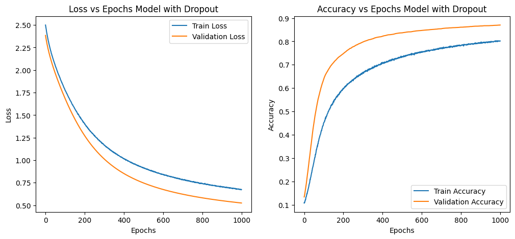
# Run an experiment with dropout
run_experiment(default_params, use_dropout=True, num_epochs=1000)
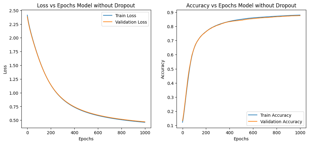
# Run an experiment without dropout
run_experiment(default_params, use_dropout=False, num_epochs=1000)Epoch 1/1000, Train Loss: 2.4997, Val Loss: 2.3846, Train Acc: 0.1074, Val Acc: 0.1335
Epoch 2/1000, Train Loss: 2.4871, Val Loss: 2.3707, Train Acc: 0.1105, Val Acc: 0.1366
Epoch 3/1000, Train Loss: 2.4759, Val Loss: 2.3572, Train Acc: 0.1087, Val Acc: 0.1408
Epoch 4/1000, Train Loss: 2.4614, Val Loss: 2.3442, Train Acc: 0.1113, Val Acc: 0.1458
Epoch 5/1000, Train Loss: 2.4476, Val Loss: 2.3318, Train Acc: 0.1145, Val Acc: 0.1513
...
Epoch 998/1000, Train Loss: 0.6720, Val Loss: 0.5255, Train Acc: 0.8023, Val Acc: 0.8700
Epoch 999/1000, Train Loss: 0.6714, Val Loss: 0.5253, Train Acc: 0.8031, Val Acc: 0.8701
Epoch 1000/1000, Train Loss: 0.6743, Val Loss: 0.5250, Train Acc: 0.8017, Val Acc: 0.8703
Test Loss: 0.5210, Test Accuracy: 0.8756
Epoch 1/1000, Train Loss: 2.4135, Val Loss: 2.3849, Train Acc: 0.1217, Val Acc: 0.1334
Epoch 2/1000, Train Loss: 2.3990, Val Loss: 2.3713, Train Acc: 0.1256, Val Acc: 0.1370
Epoch 3/1000, Train Loss: 2.3849, Val Loss: 2.3581, Train Acc: 0.1294, Val Acc: 0.1410
Epoch 4/1000, Train Loss: 2.3714, Val Loss: 2.3453, Train Acc: 0.1338, Val Acc: 0.1458
Epoch 5/1000, Train Loss: 2.3582, Val Loss: 2.3329, Train Acc: 0.1386, Val Acc: 0.1510
...
Epoch 998/1000, Train Loss: 0.4612, Val Loss: 0.4705, Train Acc: 0.8796, Val Acc: 0.8758
Epoch 999/1000, Train Loss: 0.4610, Val Loss: 0.4703, Train Acc: 0.8797, Val Acc: 0.8758
Epoch 1000/1000, Train Loss: 0.4608, Val Loss: 0.4701, Train Acc: 0.8797, Val Acc: 0.8758
Test Loss: 0.4682, Test Accuracy: 0.8784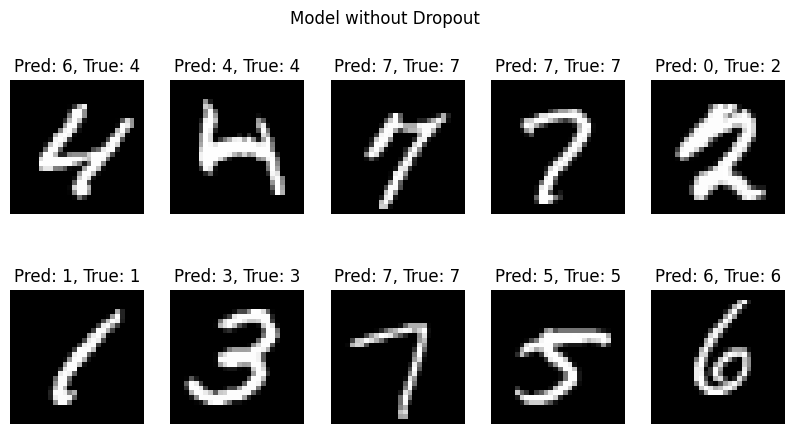
Summary of Observations
| Model Aspect | Without Dropout | With Dropout |
|---|---|---|
| Loss vs. Epochs Observation | Training and validation losses decrease steadily. | Training loss decreases more slowly; validation loss decreases more consistently. |
| Loss vs. Epochs Explanation | Indicates model learning and improving on both datasets. | Dropout forces model to be robust, leading to better generalization. |
| Accuracy vs. Epochs Observation | Both training and validation accuracies increase steadily and overlap significantly. | Validation accuracy increases and stays higher than training accuracy. |
| Accuracy vs. Epochs Explanation | Suggests potential overfitting as curves overlap. | Dropout regularizes model, preventing overfitting and improving generalization. |
Advanced Dropout Techniques
Application of Dropout after Convolution Layers
While dropout is commonly applied after fully connected layers, it can also be applied after convolutional layers. Here’s a deeper look into this practice:
Pros:
- Regularization: Helps in regularizing the model and preventing overfitting by randomly deactivating certain features.
- Improved Generalization: Encourages the model to rely on more distributed representations, improving generalization.
Cons:
- Reduced Capacity: Can significantly reduce the model’s ability to learn spatial hierarchies and patterns, as important spatial information might be lost.
- Training Complexity: Requires careful tuning to avoid underfitting, especially in deep networks where spatial hierarchies are crucial.
Use Case:
- PyTorch’s Dropout2d: This function is specifically designed for applying dropout after convolution layers. It drops entire channels (feature maps) instead of individual neurons, preserving spatial consistency.
import torch.nn as nn
class ConvNetWithDropout(nn.Module):
def __init__(self):
super(ConvNetWithDropout, self).__init__()
self.conv1 = nn.Conv2d(in_channels=3, out_channels=64, kernel_size=3, stride=1, padding=1)
self.dropout2d = nn.Dropout2d(p=0.5)
self.fc1 = nn.Linear(64 * 32 * 32, 10)
def forward(self, x):
x = self.conv1(x)
x = nn.ReLU()(x)
x = self.dropout2d(x)
x = x.view(x.size(0), -1)
x = self.fc1(x)
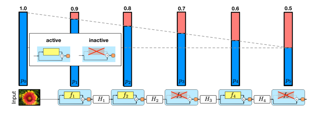
return xStochastic Depth
Stochastic depth involves randomly dropping out entire layers of a neural network during training, which can be particularly effective for very deep networks. This technique allows for layers to be skipped during training while maintaining the expected depth of the network during inference.
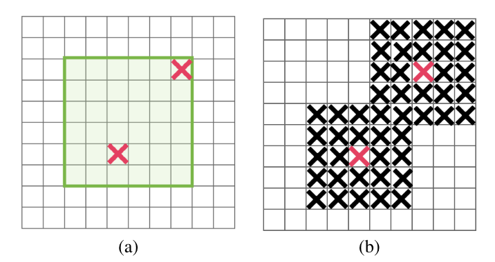
DropBlock
DropBlock is a regularization method where contiguous blocks of neurons are dropped instead of individual neurons. This method is particularly effective for convolutional neural networks (CNNs) as it maintains the spatial structure of feature maps.
Dropout for Estimating Prediction Confidence
Monte Carlo (MC) Dropout is a technique that leverages dropout to estimate prediction confidence or uncertainty in neural networks. Here’s a breakdown of how it functions:
- During training, dropout randomly deactivates (sets to zero) a fraction of neurons in each layer, which helps prevent overfitting.
- At inference time, instead of using fixed weights, multiple stochastic forward passes are performed through the network with dropout still enabled.
For each forward pass, different neurons are dropped out, leading to different predictions. The variation across these predictions provides an estimate of the model’s uncertainty. Specifically:
- The mean of these stochastic predictions represents the expected prediction value.
- The variance of these predictions approximates the model’s predictive uncertainty or confidence interval around the mean prediction. A higher variance indicates lower confidence.
The key idea is that dropout approximates a Bayesian neural network by sampling from the implicit distribution over models/weights created by the dropout masks during training. Each stochastic forward pass acts as a sample from this approximate posterior distribution.
In summary, by keeping dropout enabled during inference and performing multiple stochastic forward passes, we can estimate both the expected prediction value and its uncertainty, all without altering the existing neural network architecture. This provides a straightforward way to quantify a model’s confidence on new inputs.
How It Works
- Enable Dropout During Inference: Normally, dropout is disabled during inference. For Monte Carlo Dropout, we enable dropout during inference to introduce randomness.
- Perform Multiple Forward Passes: Run the input data through the model multiple times (e.g., 100 times) with dropout enabled each time.
- Collect Predictions: Gather the predictions from each forward pass.
- Analyze Variance: Calculate the mean and variance of the predictions. The variance provides an estimate of the model’s uncertainty.
By following these steps, Monte Carlo Dropout effectively transforms a standard neural network into a tool for uncertainty quantification, enhancing the reliability and interpretability of the model’s predictions.
Example Implementation in PyTorch
Define a Model with Dropout:
import torch
import torch.nn as nn

class SimpleNNWithDropout(nn.Module):
    def __init__(self, input_size, hidden_size, output_size, dropout_rate=0.5):
        """
        Initializes the SimpleNNWithDropout.

        Args:
            input_size (int): The number of input features.
            hidden_size (int): The number of neurons in the hidden layer.
            output_size (int): The number of output features (e.g., number of classes).
            dropout_rate (float): The probability of dropping a neuron during training.
        """
        super(SimpleNNWithDropout, self).__init__()
        # Define the first fully connected layer
        self.fc1 = nn.Linear(input_size, hidden_size)
        # Define the dropout layer
        self.dropout = nn.Dropout(dropout_rate)
        # Define the second fully connected layer
        self.fc2 = nn.Linear(hidden_size, output_size)

    def forward(self, x):
        """
        Defines the forward pass of the network.

        Args:
            x (torch.Tensor): Input tensor of shape (batch_size, input_size).

        Returns:
            torch.Tensor: Output tensor of shape (batch_size, output_size).
        """
        # Apply the first fully connected layer followed by ReLU activation
        x = torch.relu(self.fc1(x))
        # Apply dropout to the hidden layer's output during training
        x = self.dropout(x)
        # Apply the second fully connected layer
        x = self.fc2(x)
        return x
Function to Perform Monte Carlo Dropout:
def mc_dropout_inference(model, X, num_samples=100):
    """
    Performs Monte Carlo Dropout inference on the given model.

    Args:
        model (nn.Module): The neural network model with dropout layers.
        X (torch.Tensor): The input data tensor.
        num_samples (int, optional): The number of forward passes to perform. Defaults to 100.

    Returns:
        torch.Tensor: The mean of the predictions.
        torch.Tensor: The variance of the predictions.
    """
    # Set the model to training mode to enable dropout during inference
    model.train()
    predictions = []

    # Perform multiple forward passes with dropout enabled
    with torch.no_grad():  # Disable gradient calculation for inference
        for _ in range(num_samples):
            preds = model(X)  # Perform a forward pass
            predictions.append(preds)  # Store the predictions

    # Stack the predictions to create a tensor of shape (num_samples, batch_size, output_size)
    predictions = torch.stack(predictions)

    # Compute the mean of the predictions along the first dimension (num_samples)
    prediction_mean = predictions.mean(dim=0)

    # Compute the variance of the predictions along the first dimension (num_samples)
    prediction_variance = predictions.var(dim=0)

return prediction_mean, prediction_varianceVisualization:
def visualize_predictions(prediction_mean, prediction_variance):
    """
    Visualizes the prediction mean and variance to understand model confidence.

    Args:
        prediction_mean (torch.Tensor): The mean of the predictions.
        prediction_variance (torch.Tensor): The variance of the predictions.
    """
    prediction_mean = prediction_mean.numpy()
    prediction_variance = prediction_variance.numpy()

    x = np.arange(len(prediction_mean))

    plt.figure(figsize=(14, 7))

    plt.subplot(1, 2, 1)
    plt.plot(x, prediction_mean, 'o-', label='Prediction Mean')
    plt.fill_between(x, prediction_mean.squeeze() - prediction_variance.squeeze(),
                     prediction_mean.squeeze() + prediction_variance.squeeze(), alpha=0.2, label='Variance')
    plt.xlabel('Sample Index')
    plt.ylabel('Prediction Mean')
    plt.title('Prediction Mean with Variance')
    plt.legend()

    plt.subplot(1, 2, 2)
    plt.plot(x, prediction_variance, 'o-', label='Prediction Variance')
    plt.xlabel('Sample Index')
    plt.ylabel('Prediction Variance')
    plt.title('Prediction Variance')
    plt.legend()

    plt.tight_layout()
    plt.show()
Example Usage:
# Instantiate the model with specified input size, hidden size, output size, and dropout rate
input_size = 1000
hidden_size = 5
output_size = 1
dropout_rate = 0.5
model = SimpleNNWithDropout(input_size, hidden_size, output_size, dropout_rate)

# Example input data: Batch of 10 samples, each with 10 features
X = torch.randn(15, input_size)

# Perform Monte Carlo Dropout inference with 100 samples
prediction_mean, prediction_variance = mc_dropout_inference(model, X, num_samples=100)

# Print the mean and variance of the predictions
print("Prediction Mean:\n", prediction_mean)
print("Prediction Variance:\n", prediction_variance)

# Visualize the predictions to understand model confidence
visualize_predictions(prediction_mean, prediction_variance)
Prediction Mean:
tensor([[-0.3939], [-0.0638], [-0.1824], [-0.4029], [ 0.0948], [-0.3936], [-0.2374], [-0.5059], [-0.3644], [-0.3786], [ 0.2430], [-0.1282], [-0.3359], [-0.2841], [-0.3332]])
Prediction Variance:
tensor([[2.6583e-03], [8.2204e-02], [1.2063e-01], [7.4990e-03], [2.3548e-01], [3.9194e-03], [7.4403e-02], [2.0963e-02], ...[1.7139e-01], [6.3152e-06], [4.9723e-03], [0.0000e+00]])Code language: CSS (css)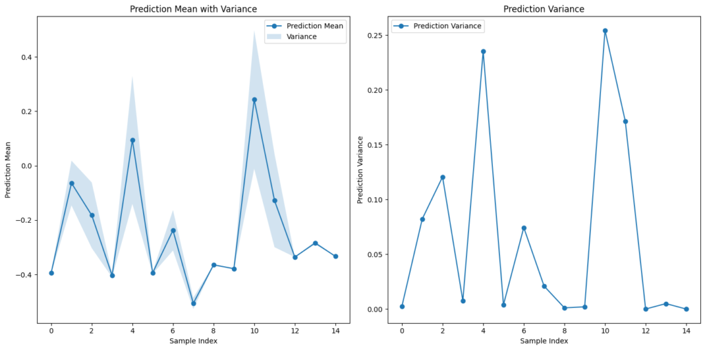
Use Cases
Uncertainty Estimation
Monte Carlo Dropout can be used to estimate the uncertainty of predictions, which is crucial in fields like healthcare and autonomous driving where the cost of wrong predictions is high. Knowing the confidence level of each prediction helps in making more informed and safer decisions.
Active Learning
In active learning scenarios, uncertainty estimates can help identify which samples the model is most uncertain about, guiding data collection for further training. This can improve the model’s performance by focusing on areas where it lacks confidence, thus making the training process more efficient and effective.
Monte Carlo Dropout is a powerful technique to estimate the prediction confidence of neural networks. By enabling dropout during inference and performing multiple forward passes, we can obtain a measure of uncertainty, which can be critical for making reliable and informed decisions based on model predictions. This approach enhances the trustworthiness and robustness of the model, especially in high-stakes applications.
Conclusion
In conclusion, dropout and its advanced variants, such as Monte Carlo Dropout, DropBlock, and Stochastic Depth, play crucial roles in enhancing the performance and generalization of neural networks. These techniques effectively address overfitting, a common challenge in machine learning models, by introducing controlled randomness during training. This forces the network to develop robust, generalized patterns rather than memorizing the training data.
Monte Carlo Dropout, in particular, extends the utility of dropout by estimating prediction uncertainty, which is invaluable in high-stakes fields like healthcare and autonomous driving. By enabling dropout during inference and performing multiple forward passes, we can quantify the model’s confidence in its predictions, leading to more informed and reliable decision-making.
Advanced techniques like DropBlock and Stochastic Depth further improve regularization, especially in convolutional neural networks and very deep architectures. These methods help maintain spatial consistency and training efficiency while enhancing the network’s generalization capabilities.
By integrating these techniques, practitioners can build more robust, reliable, and interpretable neural networks, capable of performing well on both training and unseen data. This comprehensive approach not only boosts model performance but also instills greater confidence in the predictions, paving the way for more dependable and effective machine learning applications.
References
- Srivastava, N., Hinton, G., Krizhevsky, A., Sutskever, I., & Salakhutdinov, R. (2014). Dropout: A Simple Way to Prevent Neural Networks from Overfitting. Journal of Machine Learning Research, 15, 1929-1958. Retrieved from http://jmlr.org/papers/v15/srivastava14a.html
- Huang, G., Sun, Y., Liu, Z., Sedra, D., & Weinberger, K. Q. (2016). Deep Networks with Stochastic Depth. In Proceedings of the European Conference on Computer Vision (ECCV), 646-661. Retrieved from https://arxiv.org/abs/1603.09382
- Ghiasi, G., Lin, T. Y., & Le, Q. V. (2018). DropBlock: A Regularization Method for Convolutional Networks. In Advances in Neural Information Processing Systems (NeurIPS), 31, 10750-10760. Retrieved from https://arxiv.org/abs/1810.12890
- Goodfellow, I., Bengio, Y., & Courville, A. (2016). Deep Learning. MIT Press. Retrieved from https://www.deeplearningbook.org/
- Ng, A. (2017). Deep Learning Specialization. Coursera. Retrieved from https://www.coursera.org/specializations/deep-learning
- PyTorch Documentation. (n.d.). Dropout. Retrieved from https://pytorch.org/docs/stable/nn.html#dropout
- TensorFlow Documentation. (n.d.). Dropout. Retrieved from https://www.tensorflow.org/api_docs/python/tf/keras/layers/Dropout
- Gal, Y., & Ghahramani, Z. (2016). Dropout as a Bayesian Approximation: Representing Model Uncertainty in Deep Learning. In Proceedings of the 33rd International Conference on Machine Learning (ICML), 1050-1059. Retrieved from http://proceedings.mlr.press/v48/gal16.pdf
- Reddit. (n.d.). Using Dropout for Predictions to Get a Confidence Estimate. Retrieved from https://www.reddit.com/r/datascience/comments/xq167p/using_dropout_for_predictions_to_get_a_confidence/
- Towards Data Science. (2019). Uncertainty Estimation for Neural Network: Dropout as Bayesian Approximation. Retrieved from https://towardsdatascience.com/uncertainty-estimation-for-neural-network-dropout-as-bayesian-approximation-7d30fc7bc1f2
- Xu, W. (2019). Dropout Tutorial in PyTorch. Retrieved from https://xuwd11.github.io/Dropout_Tutorial_in_PyTorch/
- Stack Overflow. (2017). How to Calculate Prediction Uncertainty Using Keras. Retrieved from https://stackoverflow.com/questions/43529931/how-to-calculate-prediction-uncertainty-using-keras