Introduction

One of the simplest ways to simulate overfitting is to use polynomial regression on a small dataset. We can fit a high-degree polynomial to a small dataset, which will lead to overfitting. Then we can see how regularization techniques like Ridge Regression (L2 regularization) help to mitigate the overfitting.

Step 1: Generate a Small Dataset

First, let’s generate a small dataset and train a neural network that will likely overfit the data.

We will generate a small dataset where y = X^2 + noise. This is a simple quadratic relationship with some added noise.

import numpy as np
import matplotlib.pyplot as plt

# Generate a small dataset
np.random.seed(42)
X = np.linspace(-1, 1, 60)
y = X**2 + np.random.randn(60) * 2

print(f'X Shape: {X.shape}')
print(f'y Shape: {y.shape}\n')

print(f'X: {X}')
print(f'y: {y}')

X Shape: (60,)
y Shape: (60,)

X: [-1.         -0.96610169 -0.93220339 -0.89830508 -0.86440678 -0.83050847
 -0.79661017 -0.76271186 -0.72881356 -0.69491525 -0.66101695 -0.62711864
 -0.59322034 -0.55932203 -0.52542373 -0.49152542 -0.45762712 -0.42372881
 -0.38983051 -0.3559322  -0.3220339  -0.28813559 -0.25423729 -0.22033898
 -0.18644068 -0.15254237 -0.11864407 -0.08474576 -0.05084746 -0.01694915
  0.01694915  0.05084746  0.08474576  0.11864407  0.15254237  0.18644068
  0.22033898  0.25423729  0.28813559  0.3220339   0.3559322   0.38983051
  0.42372881  0.45762712  0.49152542  0.52542373  0.55932203  0.59322034
  0.62711864  0.66101695  0.69491525  0.72881356  0.76271186  0.79661017
  0.83050847  0.86440678  0.89830508  0.93220339  0.96610169  1.        ]
y: [ 1.99342831  0.65682388  2.16438024  3.85301174  0.27889233  0.22147041
  3.79301339  2.11659885 -0.40777957  1.5680273  -0.48989198 -0.53818171
  0.83583491 -3.51371935 -3.17376557 -0.88297782 -1.81623966  0.80804077
 -1.66408033 -2.69791967  3.03500337 -0.36853048  0.19969301 -2.8009471
 -1.05400532  0.24511435 -2.28791074  0.75857788 -1.19869192 -0.58310023
 -1.20312595  3.70714183 -0.01981261 -2.10134544  1.668359   -2.40692717
  0.46627646 -3.85470365 -2.57334998  0.4974283   1.60362089  0.49470439
 -0.05175046 -0.39278481 -2.71544674 -1.16361832 -0.6084364   2.46615482
  1.08051437 -3.0891369   1.13107515 -0.23899536 -0.77211461  1.85794034
  2.75174337  2.60975932 -0.87148302  0.25057841  1.59587935  2.95109025]

# Plot the dataset
plt.scatter(X, y, color='blue')
plt.title('Small Dataset')
plt.xlabel('X')
plt.ylabel('y')
plt.show()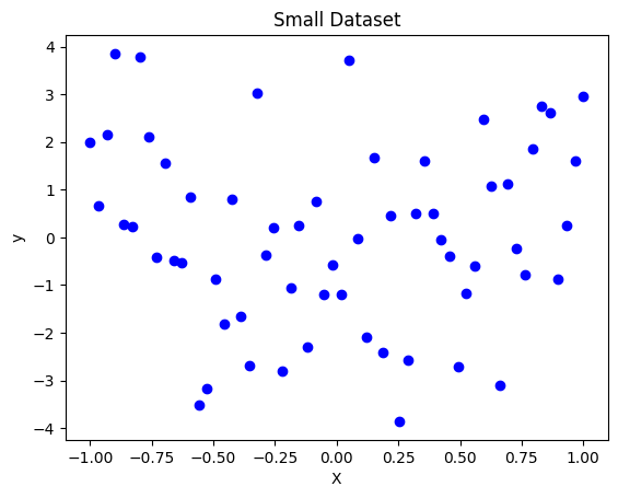

Step 2: Fit a High-Degree Polynomial

Creating Polynomial Features

from sklearn.preprocessing import PolynomialFeatures

# Create polynomial features
poly_features = PolynomialFeatures(degree=15)
X_poly = poly_features.fit_transform(X.reshape(-1, 1))
print(f'X_poly Shape: {X_poly.shape}')

X_poly Shape: (60, 16)

1- poly_features = PolynomialFeatures(degree=15): This creates an instance of PolynomialFeatures with the degree set to 15.. This means it will generate polynomial features up to the $15th$ degree. For example, if the input feature is $x$, it will generate features $1,x,x^2,x^3,…,x^{15}$.

2- X_poly = poly_features.fit_transform(X.reshape(-1, 1)):

• X.reshape(-1, 1): This reshapes the input feature array X to a 2D array with one column (60, 1). The -1 means the number of rows is inferred based on the input size.
• poly_features.fit_transform(X.reshape(-1, 1)): This method first fits the PolynomialFeatures transformer to the data X and then transforms X into a new feature matrix X_poly that contains the original features and their polynomial combinations up to the specified degree (15 in this case).

Training and Prediction

from sklearn.linear_model import LinearRegression

# Fit a linear regression model
model = LinearRegression()
model.fit(X_poly, y)

# Predict
y_pred = model.predict(X_poly)
print(f'y_pred Shape: {y_pred.shape}')

y_pred Shape: (60,)

1- fit(X_poly, y): This is the training step. Here’s what happens during this step:

• The model learns the relationship between the input features (X_poly) and the target variable (y).
• It estimates the coefficients (weights) for each feature in X_poly that minimize the error between the predicted values and the actual target values (y). This is typically done using methods like Ordinary Least Squares

2- predict(X_poly): After the model is trained, this method uses the learned coefficients to make predictions on the input data (X_poly). The predicted values are stored in y_pred.

print(f'y_pred: {y_pred}')

y_pred: [ 1.78904912  1.40950038  1.88346137  2.03553646  1.94073217  1.81354631
  1.70798893  1.54640111  1.22841837  0.71288828  0.04430492 -0.66674565
 -1.28660681 -1.70320828 -1.85742608 -1.75460089 -1.45688069 -1.06187292
 -0.67527663 -0.38506519 -0.24305829 -0.25710803 -0.39432711 -0.59336913
 -0.78210711 -0.89632865 -0.89527163 -0.77081389 -0.54864915 -0.2815172
 -0.03619069  0.12282772  0.14928545  0.0272675  -0.22343637 -0.55018789
 -0.8783894  -1.12844428 -1.23530359 -1.16615971 -0.93172534 -0.58740249
 -0.2225043   0.06164288  0.18081021  0.0973818  -0.15850241 -0.48515933
 -0.72958153 -0.73292508 -0.39410056  0.26625357  1.06954225  1.70488566
  1.8456078   1.35852475  0.54440205  0.22689037  1.30077841  3.02172261]

# Plot the results
plt.scatter(X, y, color='blue', label='Data')
plt.plot(X, y_pred, color='red', label='Overfitted Model')
plt.title('Overfitting with High-Degree Polynomial')
plt.xlabel('X')
plt.ylabel('y')
plt.legend()
plt.show()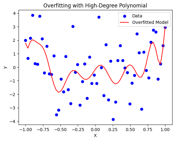

• We created a polynomial features up to the 15th degree, which introduces a lot of complexity.
• We fit a linear regression model to these polynomial features, leading to overfitting because the model is too complex for the small dataset.

Step 3: Apply Ridge Regression

from sklearn.linear_model import Ridge

# Fit a ridge regression model
ridge_model = Ridge(alpha=1, solver='cholesky')
ridge_model.fit(X_poly, y)

# Predict
y_ridge_pred = ridge_model.predict(X_poly)
print(f'y_ridge_pred Shape: {y_ridge_pred.shape}')

y_ridge_pred Shape: (60,)

1- Ridge(alpha=1, solver='cholesky'):

• Ridge: This creates an instance of the Ridge regression model.
• alpha=1: This parameter controls the regularization strength. A higher value of alpha increases regularization, which helps to prevent overfitting by penalizing large coefficients.
• solver='cholesky': This specifies the solver to use for the computations. The ‘cholesky’ solver is efficient for small datasets and uses the Cholesky decomposition to solve the linear system.

2- ridge_model.fit(X_poly, y): This is the training step for the ridge regression model. Here’s what happens during this step:

• The model learns the relationship between the input features (X_poly) and the target variable (y).
• It estimates the coefficients (weights) for each feature in X_poly that minimize the error between the predicted values and the actual target values (y), while also penalizing large coefficients to prevent overfitting. This is done by minimizing the sum of squared errors plus a penalty proportional to the sum of the squares of the coefficients.

3- y_ridge_pred = ridge_model.predict(X_poly): This uses the trained ridge regression model to predict the target variable y based on the polynomial features X_poly. The predict method returns the predicted values, which are stored in y_ridge_pred.

print(f'y_ridge_pred: {y_ridge_pred}')

y_ridge_pred: [ 2.10652297  1.9861319   1.77732828  1.52723874  1.26559883  1.01034802
  0.77158023  0.55429562  0.36028847  0.18941997  0.04045897 -0.08837631
 -0.19908012 -0.29365698 -0.37400834 -0.44187572 -0.49881859 -0.5462127
 -0.5852595  -0.61700099 -0.64233653 -0.66203957 -0.67677329 -0.68710466
 -0.69351682 -0.69641962 -0.69615878 -0.69302339 -0.68725231 -0.67903929
 -0.66853721 -0.65586126 -0.64109145 -0.62427421 -0.60542335 -0.58452025
 -0.5615133  -0.53631661 -0.50880777 -0.47882471 -0.44616134 -0.41056175
 -0.37171254 -0.32923272 -0.28266021 -0.23143359 -0.17486683 -0.11211382
 -0.0421175   0.0364641   0.12536645  0.22687908  0.34408321  0.48120331
  0.64412469  0.8411513   1.08410712  1.38992383  1.78290969  2.29796329]

# Plot the results
plt.scatter(X, y, color='blue', label='Data')
plt.plot(X, y_pred, color='red', label='Overfitted Model')
plt.plot(X, y_ridge_pred, color='green', label='Ridge Model')
plt.title('Overfitting vs. Ridge Regression')
plt.xlabel('X')
plt.ylabel('y')
plt.legend()
plt.show()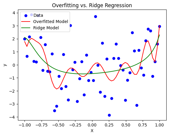

• Finally, We applied Ridge Regression (L2 regularization) with alpha = 1. This helps to penalize the coefficients of the polynomial features, reducing their magnitudes and hence the complexity of the model.
• The green line (Ridge model) should follow the general trend of the data better than the red line (overfitted model), demonstrating how regularization helps to mitigate overfitting.